Classical Test Theory
Classical test theory, also known as True Score Theory, is mainly to recognize and develop the reliability of psychological tests and assessments in psychological testing
Assumption
- The correlation between the error and the true score is 0 \(\quad \rho(T,E)=0\)
- If a person’s certain psychological trait can be repeatedly measured several times with parallel tests, the average of their observed scores will be close to the true score \(\quad\) E(X)=T
- The measurement error is random and obeys a normal random variable with the mean value of zero
- No correlation between errors on each parallel test \(\quad \rho(E_1,E_2)=0\)
CTT Model
There is a linear relationship between the observed and true fractions \[ X = T + E \] where X is observed score, T is Ture score and E is error score. Besides
Variance: \[ S^2_X= S^2_T+S^2_E \]
Limitation
- The sample dependence of statistics, the estimation of validity, reliability, difficulty, discrimination, and other parameters is very dependent on the sample, and the representativeness of the sample to the whole must be emphasized
- Test dependence of measurement scores, because it is difficult to establish “parallel papers”, the scores on two different tests measuring the same ability are not comparable.
- Imprecision of reliability estimation. CTT assumes that the measurement error is the same for subjects of different ability levels, but in fact, a test can only be administered to subjects of comparable ability level and test difficulty to obtain relatively high measurement accuracy.
Item Response Theory
Item Response Theory (IRT), also known as Latent Trait Theory or Latent Trait Model, is a modern psychometric theory that uses item characteristics to estimate latent traits in response to the limitations of CTT.
Assumption
- Unidimensionality of ability hypothesis - meaning that all items comprising a given test measure the same latent trait.
- Local independence hypothesis - meaning that no correlation exists between items for a given subject.
- Item characteristic curve hypothesis - refers to a model of the functional relationship between the probability of a subject’s correct response to an item and his or her ability.
Item Difficulty and Item Characteristic Cure
Logistic Cure or Item characteristic cure (ICC), is a function relating the probability of correct response to the ability scale.
\[P_i(\theta)=P(U_i=1|\theta)\]
To include the covariates
\[P(U_i|\theta,b_i)=\frac{e^{\theta-b_i}}{1+e^{\theta-b_i}}\]
where \(b_i\) is the item difficulty parameter.
Example:
\[P_1(\theta)=\frac{e^{\theta+1}}{1+e^{\theta+1}}, \quad P_2(\theta)=\frac{e^{\theta-1}}{1+e^{\theta-1}}\] 一条逻辑曲线就是一套试题
When \(\theta=b_i\), we say that the ability match the difficulty of the tests and we say \(P_i=0.5\).
In practice, we set \(b_i \in (-3,3)\). The larger \(b_i\), the harder item.
Outfit
Does the model fit the data well?
Residual-based fit statistics
\[P_i(\theta)=P(U_i=1|\theta), \quad \mathbb{E}(U_{ji})=P(U_i=1|\theta=\theta_j)\]
Variance (Bernulli Distribution)
\[Var(U_{ji})=P(U_i=1|\theta_j)(1-P(U_i=1|\theta_j))=0.05\times 0.95=0.0475\] 假设A每次答对的概率是0.05,所以variance很小
如果B能力更强,答对的概率是0.43,那么对应的variance会是 \[Var(U_{ji})=P(U_i=1|\theta_j)(1-P(U_i=1|\theta_j))=0.43\times 0.57=0.2451\]
如果C是个学霸,答对的概率是0.91,variance也很小
\[Var(U_{ji})=P(U_i=1|\theta_j)(1-P(U_i=1|\theta_j))=0.91\times 0.09=0.0819\] 可以相对应的算标准差, 随着能力(\(\theta\))的变化,两边小中间大
Error Bar
When a item is ‘off-target’ (too easy or too hard for a person), the variance is relatively small.
Standardized Residual
\[Z_{ji}=\frac{U_{ji}-\mathbb{E}(U_{ji})}{\sqrt{Var(U_{ji})}}\]
Outfit Mean-square Value (MNSQ)
\[outfit_i=\frac{1}{N}\sum_{j=1}^Nz^2_{ji}\]
Under-fit (bad qustions)
There is a standard in Linacre (2006)
- \(outfit > 2\), bad question, remove
- \(1.5 - 2.0\), not too bad, acceptable
- \(0.5 - 1.5\), good question
- \(<0.5\), not very much influential, acceptable
Two-parameter logistic model
\[P_i(\theta)=\frac{e^{\theta-b_i}}{1+e^{\theta-bi}}\]
\[P_i(\theta)=\frac{e^{a_i(\theta-b_i)}}{1+e^{a_i(\theta-b_i)}}\]
- \(a_i\) is the discrimination parameter.
- \(b_i\) is the item difficulty parameter.
Rasch Model
In the Rasch model, the discrinimation parameters of two-parameter logistic models are set to 1, which are equal to the one-parameter logistic models, or they are set to the same value \(a>0\) \[P_i(\theta)=\frac{e^{a_i(\theta-b_i)}}{1+e^{a_i(\theta-b_i)}}\]
A drawback to CTT/UIRT
Classical Test Theory and Item Response Theory
Remedial Course
In traditional method such as classical test theory (CTT)/unidimensional item response theory (UIRT), teachers only use total scores abilities to compare students’ learning performance.
Moreover, some students may have the same total score but their mastering skills are differet.
In recent remedial teaching, most teachers use the same learning materials for the students whose total score below than a threshold. 缺点总结,如何改进呢?
Three-parameter Logistic Model
\[[0,1] \rightarrow [0.2,1]\]
\[P_i(\theta)=c_i+(1-c_i)\frac{e^{a_i(\theta-b_i)}}{1+e^{a_i(\theta-b_i)}}\]
- \(a_i\) discrimination parameter
- \(b_i\) item difficulty parameter
- \(c_i\) guessing parameter
MTH017 Midterm Example with R
library(CTT)
library(TAM)
library(stringi)
library(tidyverse)
library(readxl)
######setwd("~/Item_Repsone_Theoryu")
#=======
#setwd("~/Item_Repsone_Theoryu")
data1<-read_excel('mth017_mid.xlsx')
data1<-data1 %>% select(2:29)
data2<- apply(data1,2,function(x) str_sub(x,-1,-1))
answer_key<-str_sub(c('1A','2B','3B','4A','5A','6B','7D','8A','9D','10B','11A','12B','13D','14A','15C','16B','17B','18C','19C','20E','21A','22B','23C','24C','25B','26C','27D','28C'),-1,-1)
CTT_score<-score(data2,answer_key,output.scored=T)
#CTT_score$scored
library(TAM)
logit1<-tam(CTT_score$scored)Then, we can extract the results
difficulty level
logit1$xsi## xsi se.xsi
## Q1 -1.59926777 0.08281262
## Q2 -0.87725851 0.07202691
## Q3 -1.90311723 0.08976346
## Q4 -1.33502667 0.07799604
## Q5 -0.89807107 0.07223796
## Q6 -0.76986328 0.07102422
## Q7 -2.23135689 0.09919926
## Q8 -1.44079642 0.07979522
## Q9 -2.30183976 0.10151477
## Q10 -2.43094886 0.10604360
## Q11 -2.56032583 0.11097420
## Q12 -1.40918138 0.07923986
## Q13 -0.87725851 0.07202691
## Q14 -2.23135689 0.09919926
## Q15 -2.11750397 0.09568201
## Q16 0.98265790 0.07347639
## Q17 -0.71971933 0.07060485
## Q18 -0.46702688 0.06894949
## Q19 -0.20028860 0.06800319
## Q20 0.03460549 0.06783063
## Q21 1.05917803 0.07440211
## Q22 -1.06392137 0.07411938
## Q23 -1.42195321 0.07958271
## Q24 -0.27688957 0.06825164
## Q25 0.09725406 0.06793617
## Q26 1.28306039 0.07758691
## Q27 -3.04702670 0.13434881
## Q28 -0.61939615 0.07052947Mean Sum of Squares
msq.itemfit(logit1)## $itemfit
## item fitgroup Outfit Outfit_t Outfit_p Infit Infit_t
## 1 Q1 1 1.0347685 0.4818066 6.299433e-01 0.9912975 -0.17320946
## 2 Q2 2 1.1716954 3.4849119 4.922990e-04 1.1069666 3.42539202
## 3 Q3 3 1.3379417 3.4078406 6.547912e-04 1.1098902 1.92729057
## 4 Q4 4 1.0902137 1.3983988 1.619934e-01 1.0814110 2.02344514
## 5 Q5 5 1.0435298 0.9180836 3.585751e-01 1.0559496 1.80499159
## 6 Q6 6 0.9731329 -0.6066728 5.440681e-01 0.9939642 -0.20191154
## 7 Q7 7 0.9798463 -0.1487582 8.817445e-01 1.0250889 0.39061237
## 8 Q8 8 0.8053456 -3.0437477 2.336510e-03 0.9101186 -2.19142974
## 9 Q9 9 0.7943306 -1.9064873 5.658701e-02 0.9350246 -0.91924611
## 10 Q10 10 0.8831100 -0.9528263 3.406781e-01 0.9576733 -0.53949162
## 11 Q11 11 0.7714293 -1.8446576 6.508737e-02 0.9446390 -0.66089618
## 12 Q12 12 0.8423894 -2.4752825 1.331308e-02 0.9351401 -1.59405400
## 13 Q13 13 1.1888686 3.8127712 1.374173e-04 1.1169149 3.73164996
## 14 Q14 14 0.7586028 -2.3733985 1.762524e-02 0.9165098 -1.24859960
## 15 Q15 15 0.8869466 -1.1119450 2.661618e-01 0.9476972 -0.82157836
## 16 Q16 16 0.9831814 -0.3261385 7.443195e-01 0.9706989 -0.88625362
## 17 Q17 17 0.9646798 -0.8325860 4.050782e-01 0.9862963 -0.48424012
## 18 Q18 18 0.9362587 -1.7919554 7.314012e-02 0.9603251 -1.59940516
## 19 Q19 19 0.9084037 -2.9405247 3.276569e-03 0.9325556 -2.95185450
## 20 Q20 20 1.2004735 6.0935245 1.104514e-09 1.1643863 6.77364610
## 21 Q21 21 0.8718964 -2.5604157 1.045470e-02 0.9051799 -2.83538677
## 22 Q22 22 0.9740119 -0.4751644 6.346698e-01 0.9731290 -0.79567373
## 23 Q23 23 1.0107089 0.1807381 8.565731e-01 0.9998988 0.01146576
## 24 Q24 24 1.0305632 0.9296578 3.525483e-01 1.0254545 1.07482170
## 25 Q25 25 0.8715860 -4.3106993 1.627391e-05 0.8971613 -4.58780807
## 26 Q26 26 1.3231286 4.8919183 9.985788e-07 1.1084814 2.69280559
## 27 Q27 27 0.8721382 -0.7189141 4.721938e-01 0.9616159 -0.31991895
## 28 Q28 28 1.0204622 0.5202281 6.029046e-01 1.0170094 0.63717621
## Infit_p
## 1 8.624868e-01
## 2 6.139129e-04
## 3 5.394343e-02
## 4 4.302727e-02
## 5 7.107600e-02
## 6 8.399859e-01
## 7 6.960838e-01
## 8 2.842071e-02
## 9 3.579669e-01
## 10 5.895477e-01
## 11 5.086789e-01
## 12 1.109239e-01
## 13 1.902297e-04
## 14 2.118116e-01
## 15 4.113169e-01
## 16 3.754809e-01
## 17 6.282155e-01
## 18 1.097306e-01
## 19 3.158717e-03
## 20 1.255766e-11
## 21 4.577024e-03
## 22 4.262217e-01
## 23 9.908518e-01
## 24 2.824546e-01
## 25 4.479241e-06
## 26 7.085357e-03
## 27 7.490298e-01
## 28 5.240101e-01
##
## $summary_itemfit
## fit M SD
## Outfit Outfit 0.9832016 0.15345336
## Infit Infit 0.9975171 0.07384753
##
## $time
## [1] "2022-08-22 19:25:13 CST" "2022-08-22 19:25:13 CST"
##
## $CALL
## msq.itemfit(object = logit1)
##
## attr(,"class")
## [1] "msq.itemfit"plot(logit1,item=1)## Iteration in WLE/MLE estimation 1 | Maximal change 1.3867
## Iteration in WLE/MLE estimation 2 | Maximal change 0.1743
## Iteration in WLE/MLE estimation 3 | Maximal change 0.0075
## Iteration in WLE/MLE estimation 4 | Maximal change 3e-04
## Iteration in WLE/MLE estimation 5 | Maximal change 0
## ----
## WLE Reliability= 0.748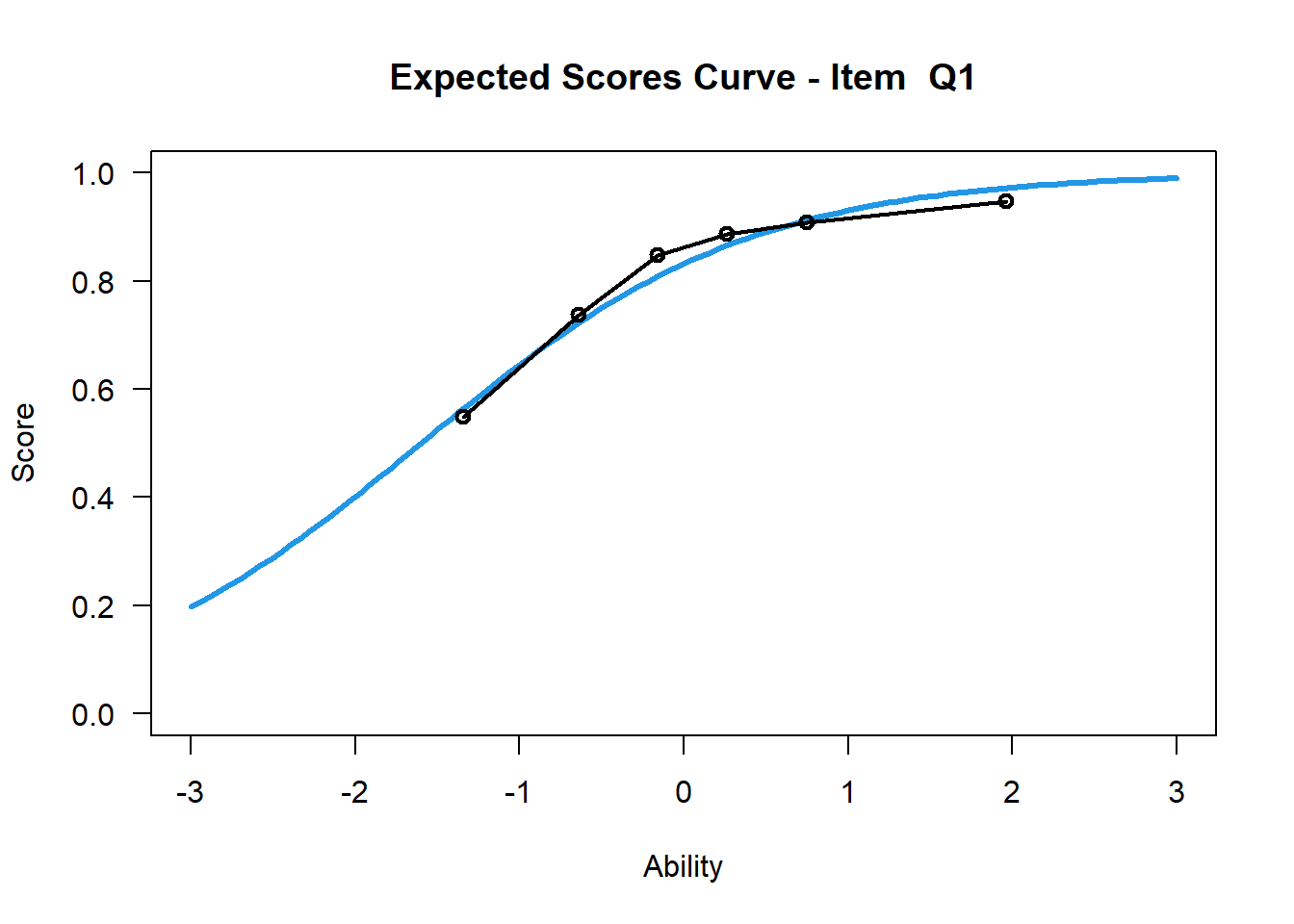
## ....................................................
##  Plots exported in png format into folder:
##  C:/Users/mu.he/Documents/Item_Repsone_Theoryu/Plots
Two Parameter IRT
logit2<-tam.mml.2pl(CTT_score$scored)logit2$item## item N M xsi.item AXsi_.Cat1 B.Cat1.Dim1
## Q1 Q1 1019 0.7998037 -1.60381101 -1.60381101 0.9007187
## Q2 Q2 1019 0.6790972 -0.78235045 -0.78235045 0.4302560
## Q3 Q3 1019 0.8400393 -1.67493255 -1.67493255 0.2209369
## Q4 Q4 1019 0.7595682 -1.21737246 -1.21737246 0.5178603
## Q5 Q5 1019 0.6830226 -0.84523068 -0.84523068 0.6661962
## Q6 Q6 1019 0.6584887 -0.77225130 -0.77225130 0.8883296
## Q7 Q7 1019 0.8763494 -2.18232206 -2.18232206 0.8048515
## Q8 Q8 1019 0.7762512 -1.87736494 -1.87736494 1.7506024
## Q9 Q9 1019 0.8832188 -2.72542893 -2.72542893 1.5053565
## Q10 Q10 1019 0.8949951 -2.72739891 -2.72739891 1.3265451
## Q11 Q11 1019 0.9057900 -3.10171074 -3.10171074 1.6050825
## Q12 Q12 1019 0.7713445 -1.65843064 -1.65843064 1.4237493
## Q13 Q13 1019 0.6790972 -0.77514562 -0.77514562 0.3790075
## Q14 Q14 1019 0.8763494 -2.80417862 -2.80417862 1.7031549
## Q15 Q15 1019 0.8645731 -2.36251740 -2.36251740 1.2899213
## Q16 Q16 1019 0.3002944 1.00989988 1.00989988 0.9982508
## Q17 Q17 1019 0.6486752 -0.76601362 -0.76601362 1.0711876
## Q18 Q18 1019 0.5976447 -0.50572989 -0.50572989 1.1007193
## Q19 Q19 1019 0.5417076 -0.23738822 -0.23738822 1.2571553
## Q20 Q20 1019 0.4916585 0.03366769 0.03366769 0.2793225
## Q21 Q21 1019 0.2865554 1.26136773 1.26136773 1.4974795
## Q22 Q22 1019 0.7134446 -1.10583136 -1.10583136 1.0118460
## Q23 Q23 1017 0.7738446 -1.43072636 -1.43072636 0.9095113
## Q24 Q24 1017 0.5585054 -0.26842353 -0.26842353 0.7575731
## Q25 Q25 1017 0.4788594 0.09734073 0.09734073 1.5325850
## Q26 Q26 1017 0.2487709 1.13862560 1.13862560 0.3651024
## Q27 Q27 1010 0.9386139 -3.42856477 -3.42856477 1.3780092
## Q28 Q28 1001 0.6313686 -0.60773020 -0.60773020 0.8094293AXsi_.Cat1 is the difficulty level
B.Cat1.Dim1 is the discrimination level
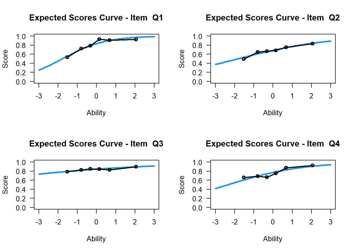
par(mfrow=c(2,2))
for(i in 1:4){
plot(logit2,items=i)
}