Sample Questions
Question 1 (10 marks)
Check the R code and results and answer the questions below.
library(ggplot2)
str(diamonds)
## tibble [53,940 × 10] (S3: tbl_df/tbl/data.frame)
## $ carat : num [1:53940] 0.23 0.21 0.23 0.29 0.31 0.24 0.24 0.26 0.22 0.23 ...
## $ cut : Ord.factor w/ 5 levels "Fair"<"Good"<..: 5 4 2 4 2 3 3 3 1 3 ...
## $ color : Ord.factor w/ 7 levels "D"<"E"<"F"<"G"<..: 2 2 2 6 7 7 6 5 2 5 ...
## $ clarity: Ord.factor w/ 8 levels "I1"<"SI2"<"SI1"<..: 2 3 5 4 2 6 7 3 4 5 ...
## $ depth : num [1:53940] 61.5 59.8 56.9 62.4 63.3 62.8 62.3 61.9 65.1 59.4 ...
## $ table : num [1:53940] 55 61 65 58 58 57 57 55 61 61 ...
## $ price : int [1:53940] 326 326 327 334 335 336 336 337 337 338 ...
## $ x : num [1:53940] 3.95 3.89 4.05 4.2 4.34 3.94 3.95 4.07 3.87 4 ...
## $ y : num [1:53940] 3.98 3.84 4.07 4.23 4.35 3.96 3.98 4.11 3.78 4.05 ...
## $ z : num [1:53940] 2.43 2.31 2.31 2.63 2.75 2.48 2.47 2.53 2.49 2.39 ...- How many kinds `cut’ of diamonds in this data set, and how many observations collected in total? How many variables(attributes) are listed in the dataset? (3 marks)
Answer: 5 kinds (1 mark), 53940 observations in the data set (1 mark), 10 variables (1 mark).
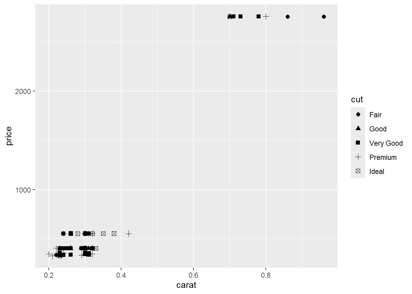
- What is the name of the package we load below, and what is the name of the plot? Hint: Scatter plot or density plot or histogram? (3 marks)
library(ggplot2) #load the package
ggplot(diamonds[1:100,], aes(x=carat, y=price, shape=cut)) + geom_point(size=2)
## Warning: Using shapes for an ordinal variable is not advised
Answer: package name: ggplot2 (1 mark), scatter plot (2 marks).
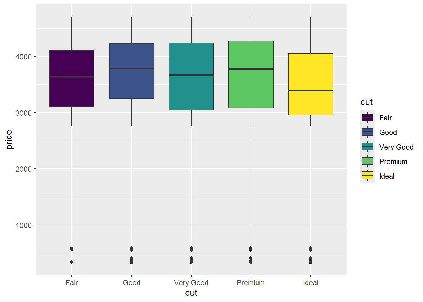
- Based on the boxplot below,
library(ggplot2)
ggplot(diamonds[1:10000,], aes(x=cut, y=price, fill=cut)) + geom_boxplot()
Compare the medians of price among different cut, give comments on the boxplot, large difference in price or not based on cut? (4 marks)
Answer: The medians are barely same, there is not large difference.
Question 2 (15 marks)
Suppose we are modeling a simple linear regression, y is the independent variable and x is the dependent variable.
x<-c(1,3,4,7,13)
y<-c(12,11,7,5,4)
cbind(x,y)
## x y
## [1,] 1 12
## [2,] 3 11
## [3,] 4 7
## [4,] 7 5
## [5,] 13 4- Write down the true model. (2 marks)
Answer: \(y=\beta_0+\beta_1x+\epsilon\) (2 marks)
- Write down the estimated model. (2 marks)
Answer: \(\hat{y}=\hat{\beta}_0+\hat{\beta}_1x\) or \(\hat{y}=b_0+b_1x\) (2 marks)
- Write down the residual. (2 marks)
Answer: \(e=y-\hat{y}\) or (\(\hat{\epsilon}=y-\hat{y}\) ) (2 marks)
- What is the assumption of the residual \(\epsilon\) (Hint: What is the distribution)? (2 marks)
Answer:
- We assume the \(\epsilon\) follows normal distribution with mean 0 and a constant standard deviation. (1 mark)
- The error terms are independent. (1 mark)
- Find the sample correlation coefficient \(r\) between \(x\) and \(y\), by the formula. (4 marks)
\[r=\frac{\sum(x-\bar{x})(y-\bar{y})}{\sqrt{\sum(x-\bar{x})^2\sum(y-\bar{y})^2}}=\frac{\sum(x-\bar{x})(y-\bar{y})}{(n-1)s_xs_y}\] (given \(\sum(x-\bar{x})(y-\bar{y})\))
Answer:
top<-sum((x-mean(x))*(y-mean(y)))
sd(x)
## [1] 4.669047sd(y)## [1] 3.563706bot<-4*sd(x)*sd(y)
top/bot## [1] -0.8774507cor(x,y)## [1] -0.8774507- Find the least square estimators \(\hat{\beta}_0\) and \(\hat{\beta}_1\), by the formula. (3 marks)
\[\hat{\beta}_1=b_1=r\frac{s_y}{s_x} , \quad \hat{\beta}_0=b_0=\bar{y}-b_1\bar{x}\] Answer:
summary(lm(y~x))##
## Call:
## lm(formula = y ~ x)
##
## Residuals:
## 1 2 3 4 5
## 1.119 1.459 -1.872 -1.862 1.156
##
## Coefficients:
## Estimate Std. Error t value Pr(>|t|)
## (Intercept) 11.5505 1.4766 7.822 0.00435 **
## x -0.6697 0.2114 -3.168 0.05054 .
## ---
## Signif. codes: 0 '***' 0.001 '**' 0.01 '*' 0.05 '.' 0.1 ' ' 1
##
## Residual standard error: 1.974 on 3 degrees of freedom
## Multiple R-squared: 0.7699, Adjusted R-squared: 0.6932
## F-statistic: 10.04 on 1 and 3 DF, p-value: 0.05054