MTH303 第 3 章：多元线性回归

MTH303 Teaching Group
School of Mathematics and Physics, XJTLU

2026-10-19

Abstract

These notes support the Chapter 3 lecture slides on multiple linear regression (MLR). They do three things that the slides state but do not derive.

Complete derivations. Starting from $SS(\bm\beta)=(\bm y-\bm X\bm\beta)^{\top}(\bm y-\bm X\bm\beta)$ we derive the normal equations, the unbiasedness of $\hat\sigma^2=\mathrm{MSE}$ , the ANOVA identity $\mathrm{TSS}=\mathrm{Reg\,SS}+\mathrm{RSS}$ , the distribution of $\mathrm{Reg\,SS}$ and $\mathrm{RSS}$ , their independence, and hence the exact null distribution $F\sim F_{p,\,n-p-1}$ of the global $F$ -statistic. The partial $F$ -test and the $t$ -test are derived as special cases, and the identity $t^2=F$ is proved.
A worked example small enough to do by hand. The fuel-use data of the slides ( $n=8$ , $p=2$ ) has a $3\times3$ $\bm X^{\top}\bm X$ whose inverse has a rational determinant ( $\det(\bm X^{\top}\bm X)=3{,}127{,}073.8$ ). Every number in the ANOVA table, the coefficient table and the residual diagnostics is computed in full.
A one-to-one check against R. For every hand-computed quantity the corresponding R command and its output are displayed, and the two are compared side by side. The companion script MTH303_Ch3_Hand_vs_R.R reproduces the whole comparison automatically and reports MATCH or DIFFERENT for each quantity.

The intended classroom sequence is: derive on the board (§（见「ANOVA 表推导」）), compute by hand in groups (§（见「手工计算例题」）), then run the R script live and watch the two columns agree (§（见「R 验证」）–§（见「教学安排与 R 脚本」）).

The Chapter 3 notes introduce $\bm H=\bm X(\bm X^{\top}\bm X)^{-1}\bm X^{\top}$ and then use it. This supplement does three things.

It exhibits the whole matrix. For the fuel-use example ( $n=8$ , $k=3$ ) all $64$ entries of $\bm H$ are printed, and then $\bm I_n-\bm H$ , whose diagonal gives the residual variances.
It proves the properties and checks each one numerically: symmetry, idempotence, $\bm H\bm X=\bm X$ , $\operatorname{rank}(\bm H)=\operatorname{tr}(\bm H)=k$ , eigenvalues in $\{0,1\}$ , and $h_{ii}=\sum_jh_{ij}^{2}$ (which is what bounds leverage between $1/n$ and $1$ ).
It rebuilds every diagnostic from $\bm H$ alone — leverage, the full residual covariance matrix $\sigma^{2}(\bm I_n-\bm H)$ , standard errors and confidence intervals, standardised and studentised residuals (both by closed form and by actually refitting the model $n$ times), Cook’s distance, the ANOVA table, the global and partial $F$ -tests, and prediction intervals. A second example with $n=45$ and $k=5$ shows that none of it depends on $n$ being small.

The companion script MTH303_Ch3_Hat_Matrix_No_Packages.R performs all of this. It calls lm() only in blocks labelled “CHECK”, and never as the source of an answer: hatvalues(), rstandard(), rstudent(), cooks.distance(), vcov(), confint() and predict() are all re-implemented from first principles and then compared with R’s own functions. All $29$ comparisons agree to at least $10^{-7}$ (most to $10^{-13}$ ); the complete transcript is in MTH303_Ch3_Hat_Matrix_Output.txt.

符号与模型Notation and the model

本节导读：先规定记法：标量形式、矩阵形式与基本假设（独立、零均值、同方差、正态）。这是后面所有推导的语言基础：学生要能默写 y = Xβ + ε，理解 k = p + 1 的含义，以及满秩条件 rank(X) = p + 1 为什么是 XᵀX 可逆的前提。

标量形式的模型The model in scalar form

With $p$ explanatory variables and $n$ independent observations, $\begin{equation} \label{eq:model} y_i=\beta_0+\beta_1x_{i1}+\beta_2x_{i2}+\cdots+\beta_px_{ip}+\varepsilon_i, \qquad i=1,\dots,n, \end{equation}$ where the errors satisfy $\begin{equation} \label{eq:assumptions} \varepsilon_1,\dots,\varepsilon_n\ \text{are independent},\qquad \mathbb{E}[\varepsilon_i]=0,\qquad \operatorname{Var}(\varepsilon_i)=\sigma^2, \end{equation}$ and, for inference, $\varepsilon_i\sim N(0,\sigma^2)$ . The quantity $\mathbb{E}[y_i\mid x_{i1},\dots,x_{ip}]=\beta_0+\beta_1x_{i1}+\cdots+\beta_px_{ip}$ is the regression function. The parameter $\beta_j$ is the change in the mean response associated with a one-unit increase in $x_j$ holding all other predictors fixed.

矩阵形式的模型The model in matrix form

Stacking the $n$ equations （见公式） gives $\begin{equation} \label{eq:matrixmodel} \underbrace{\begin{pmatrix}y_1\\y_2\\\vdots\\y_n\end{pmatrix}}_{\bm y\ (n\times1)} = \underbrace{\begin{pmatrix} 1 & x_{11} & x_{12} & \cdots & x_{1p}\\ 1 & x_{21} & x_{22} & \cdots & x_{2p}\\ \vdots & \vdots & \vdots & \ddots & \vdots\\ 1 & x_{n1} & x_{n2} & \cdots & x_{np} \end{pmatrix}}_{\bm X\ (n\times(p+1))} \underbrace{\begin{pmatrix}\beta_0\\\beta_1\\\vdots\\\beta_p\end{pmatrix}}_{\bm\beta\ ((p+1)\times1)} + \underbrace{\begin{pmatrix}\varepsilon_1\\\varepsilon_2\\\vdots\\\varepsilon_n\end{pmatrix}}_{\bm\varepsilon\ (n\times1)} . \end{equation}$ Write $k:=p+1$ for the number of regression parameters (intercept plus slopes). In compact form, $\bm y=\bm X\bm\beta+\bm\varepsilon,\qquad \mathbb{E}[\bm\varepsilon]=\bm 0,\qquad \operatorname{Var}(\bm\varepsilon)=\sigma^2\bm I_n,\qquad \bm\varepsilon\sim N_n(\bm 0,\sigma^2\bm I_n)\ \text{for inference.}$ $\bm X$ is the design matrix. In the rest of these notes $\bm X$ always contains a column of ones, so the model has an intercept; the last part of §6.13 explains what changes if it does not.

注记

Remark 1 (Full rank). All of the algebra below assumes $\operatorname{rank}(\bm X)=k=p+1$ , i.e. the columns of $\bm X$ are linearly independent. This is exactly the condition under which $\bm X^{\top}\bm X$ is invertible. It fails if, for example, one predictor is a linear combination of the others, or if a categorical predictor with $r$ levels is coded with $r$ dummy variables while an intercept is also present (the “dummy-variable trap”).

最小二乘估计Least squares estimation

本节导读：从残差平方和出发，用矩阵微积分推出正规方程与 β̂ = (XᵀX)⁻¹Xᵀy；随后给出拟合值、残差与帽子矩阵 H = X(XᵀX)⁻¹Xᵀ，并证明它们对称、幂等、迹为 k。最后证明 β̂ 无偏、协方差为 σ²(XᵀX)⁻¹，为后面的标准误公式做准备。

最小二乘准则与正规方程The least squares criterion and the normal equations

定义

Definition 2 (Least squares estimator). The least squares estimator $\hat{\bm\beta}$ minimises the residual sum of squares $\begin{equation} \label{eq:SS} SS(\bm\beta)=(\bm y-\bm X\bm\beta)^{\top}(\bm y-\bm X\bm\beta) =\sum_{i=1}^{n}\Bigl(y_i-\sum_{j=0}^{p}\beta_jx_{ij}\Bigr)^{2}, \qquad x_{i0}:=1 . \end{equation}$

Theorem 3 (Normal equations). If $\operatorname{rank}(\bm X)=p+1$ then $SS(\bm\beta)$ has the unique minimiser $\begin{equation} \label{eq:betahat} {\ \hat{\bm\beta}=(\bm X^{\top}\bm X)^{-1}\bm X^{\top}\bm y\ } \end{equation}$ and $\hat{\bm\beta}$ solves the normal equations $\bm X^{\top}\bm X\,\bm\beta=\bm X^{\top}\bm y$ .

证明

Proof. Expand the quadratic form: $\begin{equation} \label{eq:expand} SS(\bm\beta) =\bm y^{\top}\bm y-2\bm\beta^{\top}\bm X^{\top}\bm y+\bm\beta^{\top}\bm X^{\top}\bm X\bm\beta . \end{equation}$ We need two matrix-calculus facts, both obtained by writing the expression out in components and differentiating with respect to each $\beta_j$ : $\frac{\partial(\bm a^{\top}\bm\beta)}{\partial\bm\beta}=\bm a, \qquad \frac{\partial(\bm\beta^{\top}\bm A\bm\beta)}{\partial\bm\beta} =(\bm A+\bm A^{\top})\bm\beta .$ (For the second: $\bm\beta^{\top}\bm A\bm\beta=\sum_{r,s}A_{rs}\beta_r\beta_s$ , and $\partial/\partial\beta_j$ of that is $\sum_s A_{js}\beta_s+\sum_r A_{rj}\beta_r$ , which is the $j$ -th entry of $(\bm A+\bm A^{\top})\bm\beta$ .) Applying these to （见公式） with $\bm A=\bm X^{\top}\bm X$ symmetric gives the gradient $\begin{equation} \label{eq:gradient} \frac{\partial SS(\bm\beta)}{\partial\bm\beta} =-2\bm X^{\top}\bm y+2\bm X^{\top}\bm X\bm\beta =-2\bm X^{\top}(\bm y-\bm X\bm\beta). \end{equation}$ Setting this to zero gives the normal equations $\bm X^{\top}\bm X\bm\beta=\bm X^{\top}\bm y$ . Because $\operatorname{rank}(\bm X)=p+1$ , $\bm X^{\top}\bm X$ is positive definite and hence invertible, so the unique stationary point is （见公式）. Finally, the Hessian $\frac{\partial^{2}SS(\bm\beta)}{\partial\bm\beta\,\partial\bm\beta^{\top}} =2\bm X^{\top}\bm X$ is positive definite, so （见公式） is a minimum (indeed the unique global minimum, since $SS$ is a strictly convex quadratic). ◻

注记

Remark 4 (The component form of the first-order conditions). Writing the normal equations out row by row gives the familiar system $\sum_i e_i=0,\qquad \sum_i x_{i1}e_i=0,\qquad \dots,\qquad \sum_i x_{ip}e_i=0,$ where $e_i:=y_i-\hat y_i$ are the residuals and $\hat y_i=\bm x_i^{\top}\hat{\bm\beta}$ . In matrix form this is the single statement $\begin{equation} \label{eq:Xte} \bm X^{\top}\bm e=\bm 0 . \end{equation}$ Equation （见公式） is the reason the ANOVA decomposition works, so it deserves to be highlighted.

拟合值、残差与帽子矩阵Fitted values, residuals and the hat matrix

定义

Definition 5 (Fitted values, residuals, hat matrix). $\hat{\bm y}:=\bm X\hat{\bm\beta},\qquad \bm e:=\bm y-\hat{\bm y},\qquad \bm H:=\bm X(\bm X^{\top}\bm X)^{-1}\bm X^{\top}.$ $\bm H$ is called the hat matrix because $\hat{\bm y}=\bm H\bm y$ : it puts the hat on $\bm y$ .

Proposition 6 (Properties of $\bm H$ ). The matrix $\bm H$ is symmetric and idempotent: $\bm H^{\top}=\bm H$ and $\bm H^{2}=\bm H$ . Consequently $\hat{\bm y}=\bm H\bm y,\qquad \bm e=(\bm I_n-\bm H)\bm y,$ and $\bm I_n-\bm H$ is also symmetric and idempotent, $\bm H(\bm I_n-\bm H)=\bm 0$ . Moreover $\operatorname{tr}(\bm H)=\operatorname{rank}(\bm H)=p+1=k$ and hence $\operatorname{tr}(\bm I_n-\bm H)=n-k$ .

证明

Proof. Symmetry: $\bm H^{\top}=(\bm X(\bm X^{\top}\bm X)^{-1}\bm X^{\top})^{\top} =\bm X((\bm X^{\top}\bm X)^{-1})^{\top}\bm X^{\top}=\bm H$ , because $\bm X^{\top}\bm X$ and hence its inverse are symmetric. Idempotence: $\bm H^{2}=\bm X(\bm X^{\top}\bm X)^{-1}\underbrace{\bm X^{\top}\bm X(\bm X^{\top}\bm X)^{-1}}_{\bm I_n}\bm X^{\top} =\bm X(\bm X^{\top}\bm X)^{-1}\bm X^{\top}=\bm H.$ Then $\bm e=\bm y-\bm X\hat{\bm\beta}=(\bm I_n-\bm H)\bm y$ , and $(\bm I_n-\bm H)^{2}=\bm I_n-2\bm H+\bm H^{2}=\bm I_n-\bm H$ . Finally, for any idempotent matrix $\operatorname{tr}(\bm H)=\operatorname{rank}(\bm H)$ ; and $\operatorname{rank}(\bm H)=\operatorname{rank}(\bm X)=p+1$ because $\bm H$ is the orthogonal projector onto the column space of $\bm X$ . Hence $\operatorname{tr}(\bm I_n-\bm H)=n-(p+1)=n-k$ . ◻

命题

Proposition 7 (Two consequences of the normal equations). With $\bm e=\bm y-\hat{\bm y}$ , $\begin{equation} \label{eq:orth} \bm X^{\top}\bm e=\bm 0,\qquad\text{so}\qquad \sum_{i=1}^{n}e_i=0 \quad\text{and}\quad \sum_{i=1}^{n}\hat y_ie_i=0, \end{equation}$ and $\begin{equation} \label{eq:pythagoras} \hat{\bm y}^{\top}\hat{\bm y}+\bm e^{\top}\bm e=\bm y^{\top}\bm y, \qquad\text{i.e.}\qquad \sum_i\hat y_i^{2}+\sum_ie_i^{2}=\sum_iy_i^{2}. \end{equation}$

证明

Proof. $\bm X^{\top}\bm e=\bm X^{\top}\bm y-\bm X^{\top}\bm X\hat{\bm\beta}=\bm X^{\top}\bm y-\bm X^{\top}\bm y=\bm 0$ by the normal equations. The first column of $\bm X$ is $\bm 1=(1,\dots,1)^{\top}$ , so the first entry of $\bm X^{\top}\bm e$ is $\sum_ie_i=0$ ; and $\sum_i\hat y_ie_i=\hat{\bm y}^{\top}\bm e=(\bm X\hat{\bm\beta})^{\top}\bm e=\hat{\bm\beta}^{\top}\bm X^{\top}\bm e=0$ . For （见公式）, $\bm y=\hat{\bm y}+\bm e$ and the two pieces are orthogonal, so $\bm y^{\top}\bm y=\hat{\bm y}^{\top}\hat{\bm y}+2\hat{\bm y}^{\top}\bm e+\bm e^{\top}\bm e=\hat{\bm y}^{\top}\hat{\bm y}+\bm e^{\top}\bm e$ . ◻

估计量的均值与协方差Mean and covariance of the least squares estimator

Theorem 8 (Unbiasedness and covariance). Under $\bm y=\bm X\bm\beta+\bm\varepsilon$ with $\mathbb{E}[\bm\varepsilon]=\bm 0$ and $\operatorname{Var}(\bm\varepsilon)=\sigma^{2}\bm I_n$ , $\begin{equation} \label{eq:meanvar} \mathbb{E}[\hat{\bm\beta}]=\bm\beta, \qquad \operatorname{Var}(\hat{\bm\beta})=\sigma^{2}(\bm X^{\top}\bm X)^{-1}. \end{equation}$ Moreover, if $\bm\varepsilon\sim N_n(\bm 0,\sigma^{2}\bm I_n)$ then $\begin{equation} \label{eq:betanormal} \hat{\bm\beta}\sim N_{p+1}\bigl(\bm\beta,\ \sigma^{2}(\bm X^{\top}\bm X)^{-1}\bigr). \end{equation}$

证明

Proof. First note that $\hat{\bm\beta}=\bm A\bm y$ with $\bm A=(\bm X^{\top}\bm X)^{-1}\bm X^{\top}$ , and $\bm A\bm X=(\bm X^{\top}\bm X)^{-1}\bm X^{\top}\bm X=\bm I_n$ . Hence $\mathbb{E}[\hat{\bm\beta}]=\bm A\mathbb{E}[\bm y]=\bm A\bm X\bm\beta=\bm\beta$ . For the covariance, using $\operatorname{Var}(\bm A\bm y)=\bm A\operatorname{Var}(\bm y)\bm A^{\top}$ , $\operatorname{Var}(\hat{\bm\beta})=\bm A\,\sigma^{2}\bm I_n\,\bm A^{\top} =\sigma^{2}(\bm X^{\top}\bm X)^{-1}\underbrace{\bm X^{\top}\bm X}_{}\underbrace{(\bm X^{\top}\bm X)^{-1}\bm X^{\top}\bm X}_{}\cdots =\sigma^{2}(\bm X^{\top}\bm X)^{-1},$ more concisely $\operatorname{Var}(\hat{\bm\beta})=\sigma^{2}(\bm X^{\top}\bm X)^{-1}\bm X^{\top}\bm X(\bm X^{\top}\bm X)^{-1} =\sigma^{2}(\bm X^{\top}\bm X)^{-1}.$ Finally, $\hat{\bm\beta}$ is a fixed linear transformation of the normal vector $\bm y$ , so it is normal with the mean and covariance just computed. ◻

注记

Remark 9 (Reading the covariance matrix). The $(j+1)$ -th diagonal element of $\sigma^{2}(\bm X^{\top}\bm X)^{-1}$ is $\operatorname{Var}(\hat\beta_j)$ , so the standard error of $\hat\beta_j$ is estimated by $\begin{equation} \label{eq:se} \widehat{\mathrm{se}}(\hat\beta_j) =\sqrt{\hat\sigma^{2}\,[(\bm X^{\top}\bm X)^{-1}]_{jj}} =\sqrt{\mathrm{MSE}\,[(\bm X^{\top}\bm X)^{-1}]_{jj}} , \end{equation}$ where $\mathrm{MSE}$ is defined and justified in §3.2. Off-diagonal elements are covariances, $\operatorname{Cov}(\hat\beta_j,\hat\beta_l) =\sigma^{2}[(\bm X^{\top}\bm X)^{-1}]_{jl}$ .

ANOVA 表的完整推导The ANOVA table: derivations

本节导读：本章的核心。按四个逻辑步骤拆开：（1）纯代数的分解 TSS = RegSS + RSS；（2）MSE 是 σ² 的无偏估计；（3）正态性下 RSS 与 RegSS 的 χ² 分布及相互独立；（4）由此得到整体 F 检验。要点是让学生清楚每一步分别用到了什么假设。

This is the core of the chapter. We build the ANOVA table in four logically separate steps, because it is important to see what is pure algebra and what needs the normal model:

Algebra (§3.1): the identity $\mathrm{TSS}=\mathrm{Reg\,SS}+\mathrm{RSS}$ , which holds for the least squares fit regardless of any distributional assumption.
Unbiasedness (§3.2): $\mathbb{E}[\mathrm{MSE}]=\sigma^{2}$ , which also needs only （见公式） and not normality.
Distributions (§3.3): under normality, $\mathrm{RSS}/\sigma^{2}\sim\chi^{2}_{n-k}$ , $\mathrm{Reg\,SS}/\sigma^{2}\sim\chi^{2}_{p}$ under $H_0$ , and the two are independent.
The test (§3.4): the ratio therefore has an $F$ distribution, which is the ANOVA $F$ -test.

第 1 步：ANOVA 恒等式Step 1: the ANOVA identity T S S = R e g S S + R S S

定义

Definition 10 (The three sums of squares). $\begin{align} \mathrm{TSS}&=\sum_{i=1}^{n}(y_i-\bar y)^{2} =\sum_iy_i^{2}-n\bar y^{2} =\bm y^{\top}\bm y-\tfrac1n\bm y^{\top}\bm 1\bm 1^{\top}\bm y, \label{eq:tss}\\[0.2em] \mathrm{Reg\,SS}&=\sum_{i=1}^{n}(\hat y_i-\bar y)^{2} =\sum_i\hat y_i^{2}-n\bar y^{2}, \label{eq:regss}\\[0.2em] \mathrm{RSS}&=\sum_{i=1}^{n}(y_i-\hat y_i)^{2}=\sum_ie_i^{2}=\bm e^{\top}\bm e . \label{eq:rss} \end{align}$ The total sum of squares $\mathrm{TSS}$ measures the variation of the response about its mean before regression; $\mathrm{RSS}$ is what is left over after regression; $\mathrm{Reg\,SS}$ is the part the regression has accounted for.

Theorem 11 (ANOVA decomposition). For the least squares fit of a model with an intercept, $\begin{equation} \label{eq:anovatss} {\ \mathrm{TSS}=\mathrm{Reg\,SS}+\mathrm{RSS}\ } \end{equation}$ and all three quantities are non-negative.

证明

Proof. The starting point is the elementary telescoping identity, valid for every $i$ : $\begin{equation} \label{eq:telescope} y_i-\bar y=\underbrace{(y_i-\hat y_i)}_{e_i}+\underbrace{(\hat y_i-\bar y)}_{}. \end{equation}$ Note carefully that $\bar{\hat y}=\bar y$ , because $\sum_i\hat y_i=\bm 1^{\top}\hat{\bm y}=\bm 1^{\top}\bm H\bm y$ and $\bm 1$ is a column of $\bm X$ , so $\bm H\bm 1=\bm 1$ and therefore $\sum_i\hat y_i=\bm 1^{\top}\bm y=\sum_iy_i$ . Now square （见公式） and sum over $i$ : $\mathrm{TSS}=\sum_i(y_i-\bar y)^{2} =\sum_ie_i^{2}+\sum_i(\hat y_i-\bar y)^{2} +2\sum_i e_i(\hat y_i-\bar y).$ The cross term vanishes: $\sum_i e_i(\hat y_i-\bar y) =\sum_ie_i\hat y_i-\bar y\sum_ie_i =0-0=0,$ using $\sum_i\hat y_ie_i=0$ and $\sum_ie_i=0$ from Proposition 6 (equivalently, （见公式）). Hence $\mathrm{TSS}=\mathrm{RSS}+\mathrm{Reg\,SS}$ . Non-negativity is clear from the squared-sum definitions. ◻

注记

Remark 12 (The geometric content). In matrix form the decomposition is orthogonal projection of $\bm y$ onto two orthogonal subspaces: $\hat{\bm y}=\bm H\bm y$ is the projection onto the column space of $\bm X$ (the “explained” part) and $\bm e=(\bm I_n-\bm H)\bm y$ is the projection onto its orthogonal complement (the “unexplained” part). The identity $\mathrm{TSS}=\mathrm{Reg\,SS}+\mathrm{RSS}$ is Pythagoras’ theorem in $\mathbb{R}^{n}$ , after centring. This is why （见公式） and $\sum_ie_i=0$ are the only two facts needed.

注记

Remark 13 (Two useful alternative forms). Using the normal equations $\bm X^{\top}\bm X\hat{\bm\beta}=\bm X^{\top}\bm y$ , $\begin{equation} \label{eq:regssbeta} \mathrm{Reg\,SS}=\hat{\bm\beta}^{\top}\bm X^{\top}\bm y-n\bar y^{2}=\hat{\bm\beta}^{\top}\bm X^{\top}\bm y-\tfrac1n\bm y^{\top}\bm 1\bm 1^{\top}\bm y, \end{equation}$ and, subtracting （见公式） from （见公式） and using ŷᵀŷ = yᵀy − RSS from （见公式）, $\begin{equation} \label{eq:regssalt} \mathrm{Reg\,SS}=\hat{\bm y}^{\top}\hat{\bm y}-\tfrac1n\bm y^{\top}\bm 1\bm 1^{\top}\bm y. \end{equation}$ Formulae （见公式） and （见公式） are the two versions students should be able to reproduce; the worked example of §6 checks that they agree.

第 2 步：MSE 是 σ² 的无偏估计Step 2: M S E is an unbiased estimator of σ 2

The ANOVA table divides each sum of squares by its degrees of freedom. We now justify the choice of denominator for the error line.

Lemma 14 (Expected residual sum of squares). Under $\bm y=\bm X\bm\beta+\bm\varepsilon$ with $\mathbb{E}[\bm\varepsilon]=\bm 0$ and $\operatorname{Var}(\bm\varepsilon)=\sigma^{2}\bm I_n$ , $\begin{equation} \label{eq:erss} \mathbb{E}[\mathrm{RSS}]=\mathbb{E}[\bm e^{\top}\bm e]=\sigma^{2}(n-p-1)=\sigma^{2}(n-k). \end{equation}$

证明

Proof. Since $\bm e=(\bm I_n-\bm H)\bm y=(\bm I_n-\bm H)\bm\varepsilon$ (because $(\bm I_n-\bm H)\bm X\bm\beta=\bm 0$ ), we have $\bm e^{\top}\bm e=\bm\varepsilon^{\top}(\bm I_n-\bm H)^{\top}(\bm I_n-\bm H)\bm\varepsilon =\bm\varepsilon^{\top}(\bm I_n-\bm H)\bm\varepsilon$ , using symmetry and idempotence of $\bm I_n-\bm H$ . For a quadratic form in a random vector with mean $\bm\mu$ and covariance $\bm\Sigma$ , $\mathbb{E}[\bm\varepsilon^{\top}\bm M\bm\varepsilon]=\operatorname{tr}(\bm M\bm\Sigma)+\bm\mu^{\top}\bm M\bm\mu .$ (This follows by writing $\bm\varepsilon^{\top}\bm M\bm\varepsilon=\sum_{r,s}M_{rs}\varepsilon_r\varepsilon_s$ and using $\mathbb{E}[\varepsilon_r\varepsilon_s]=\Sigma_{rs}+\mu_r\mu_s$ .) Applying it with $\bm M=\bm I_n-\bm H$ , $\bm\Sigma=\sigma^{2}\bm I_n$ , $\bm\mu=\bm 0$ , $\mathbb{E}[\bm e^{\top}\bm e]=\sigma^{2}\operatorname{tr}(\bm I_n-\bm H)=\sigma^{2}\bigl(n-\operatorname{tr}(\bm H)\bigr) =\sigma^{2}(n-p-1),$ because $\operatorname{tr}(\bm H)=p+1$ by Proposition 6. ◻

Corollary 15 (The ANOVA table is built from unbiased quantities). Define $\mathrm{MSE}:=\frac{\mathrm{RSS}}{n-p-1},\qquad \mathrm{MSR}:=\frac{\mathrm{Reg\,SS}}{p},\qquad s^{2}:=\mathrm{MSE}.$ Then $\mathbb{E}[\mathrm{MSE}]=\sigma^{2}$ : the error mean square is an unbiased estimator of the error variance. Equivalently, $s=\sqrt{\mathrm{MSE}}$ is the “residual standard error” reported by summary() in R. Also, under $H_0:\beta_1=\cdots=\beta_p=0$ one has $\mathbb{E}[\mathrm{MSR}]=\sigma^{2}$ .

证明

Proof. The first claim is Lemma 14 divided by $n-p-1$ . For the second, under $H_0$ the regression function is the constant $\beta_0$ , so the fitted values converge to $\bar y$ and $\mathbb{E}[\mathrm{Reg\,SS}]=\mathbb{E}[\mathrm{TSS}]-\mathbb{E}[\mathrm{RSS}]$ . With $\mathbb{E}[\mathrm{TSS}]=(n-1)\sigma^{2}$ (the usual unbiased variance numerator) we get $\mathbb{E}[\mathrm{Reg\,SS}]=(n-1)\sigma^{2}-(n-p-1)\sigma^{2} =p\sigma^{2}$ , hence $\mathbb{E}[\mathrm{MSR}]=\sigma^{2}$ . ◻

注记

Remark 16 (Why the degrees of freedom are what they are). The ANOVA table below divides by $p$ , $n-p-1$ and $n-1$ . The counting rule is:

$\mathrm{TSS}$ has $n-1$ df: $n$ observations, minus one for the estimated mean $\bar y$ .
$\mathrm{RSS}$ has $n-p-1$ df: $n$ observations, minus $p+1$ for the estimated parameters $\hat\beta_0,\dots,\hat\beta_p$ . Algebraically, $\operatorname{rank}(\bm I_n-\bm H)=n-p-1$ .
$\mathrm{Reg\,SS}$ has $p$ df: the leftover $(n-1)-(n-p-1)=p$ , the number of slopes being tested. Algebraically, the centred fitted vector $(\hat y_1-\bar y,\dots)$ lives in a $p$ -dimensional space.

Degrees of freedom therefore also add: $p+(n-p-1)=n-1$ .

第 3 步：RSS 与 RegSS 的分布及其独立性Step 3: distribution of R S S and R e g S S , and their independence

Now normality enters. The tool is Cochran’s theorem in a form that is easy to verify directly.

Lemma 17 (Distribution of a quadratic form). Let $\bm z\sim N_n(\bm 0,\bm I_n)$ and let $\bm A$ be symmetric and idempotent with $\operatorname{rank}(\bm A)=r$ . Then $\bm z^{\top}\bm A\bm z\sim\chi^{2}_{r}.$ Moreover, if $\bm B$ is symmetric and idempotent with $\bm A\bm B=\bm 0$ , then $\bm z^{\top}\bm A\bm z$ and $\bm z^{\top}\bm B\bm z$ are independent.

证明

Proof sketch. Write the spectral decomposition $\bm A=\bm P\bm\Lambda\bm P^{\top}$ , with $\bm P$ orthogonal and $\bm\Lambda=\mathrm{diag}(\lambda_1,\dots,\lambda_n).$ Symmetry plus idempotence forces every eigenvalue to satisfy $\lambda^{2}=\lambda$ , so $\lambda_j\in\{0,1\}$ , and $\operatorname{rank}(\bm A)=\sum_j\lambda_j=r$ (the number of unit eigenvalues). Then $\bm z^{\top}\bm A\bm z=\sum_{j=1}^{n}\lambda_j(\bm P^{\top}\bm z)_j^{2} =\sum_{j:\,\lambda_j=1}w_j^{2}, \qquad \bm w=\bm P^{\top}\bm z\sim N_n(\bm 0,\bm I_n),$ a sum of $r$ independent squared standard normals, i.e. $\chi^{2}_r$ . If in addition $\bm A\bm B=\bm 0$ then the columns of $\bm P$ belonging to unit eigenvalues of $\bm A$ are orthogonal to those belonging to unit eigenvalues of $\bm B$ , so the two sums involve disjoint groups of the independent $w_j$ ; independence follows. ◻

Theorem 18 (Distributions behind the ANOVA table). Assume $\bm\varepsilon\sim N_n(\bm 0,\sigma^{2}\bm I_n)$ and $\operatorname{rank}(\bm X)=p+1=k$ . Then $\begin{align} \frac{\mathrm{RSS}}{\sigma^{2}}&\sim\chi^{2}_{\,n-p-1}, \qquad\text{and}\qquad \mathrm{RSS}\ \text{is independent of}\ \hat{\bm\beta} \nonumber\\&\qquad\qquad\qquad\qquad\text{(hence of }\hat{\bm y}\ \text{and }\mathrm{Reg\,SS}\text{)}. \label{eq:rssdist}\\[0.4em] \text{Under }H_0:\beta_1&=\cdots=\beta_p=0:\qquad \frac{\mathrm{Reg\,SS}}{\sigma^{2}}\sim\chi^{2}_{\,p}, \qquad\text{and}\qquad \mathrm{Reg\,SS}\ \perp\!\!\!\perp\ \mathrm{RSS}. \label{eq:regssdist} \end{align}$

证明

Proof. (a) The error line. Put $\bm z=\bm\varepsilon/\sigma\sim N_n(\bm 0,\bm I_n)$ . Because $(\bm I_n-\bm H)\bm X=\bm 0$ , $\bm e=(\bm I_n-\bm H)\bm y=(\bm I_n-\bm H)\bm\varepsilon=\sigma(\bm I_n-\bm H)\bm z .$ The matrix $\bm I_n-\bm H$ is symmetric and idempotent with rank $n-k$ by Proposition 6, so Lemma 17 gives $\frac{\mathrm{RSS}}{\sigma^{2}}=\bm z^{\top}(\bm I_n-\bm H)\bm z\sim\chi^{2}_{n-k}.$

(b) Independence of （见公式）. Since $\bm e$ and $\hat{\bm\beta}$ are linear in $\bm y$ , the pair $(\bm e,\hat{\bm\beta})$ is jointly normal. Joint normality plus zero covariance implies independence, so it suffices to show $\operatorname{Cov}(\bm e,\hat{\bm\beta})=\bm 0$ : $\operatorname{Cov}\bigl((\bm I_n-\bm H)\bm y,\ \bm A\bm y\bigr) =(\bm I_n-\bm H)\,\sigma^{2}\bm I_n\,\bm A^{\top} =\sigma^{2}(\bm I_n-\bm H)\bm A^{\top}, \qquad \bm A=(\bm X^{\top}\bm X)^{-1}\bm X^{\top}.$ Now $\bm A^{\top}=\bm X(\bm X^{\top}\bm X)^{-1}$ , so $(\bm I_n-\bm H)\bm A^{\top} =\bm X(\bm X^{\top}\bm X)^{-1}-\bm X(\bm X^{\top}\bm X)^{-1}\bm X^{\top}\bm X(\bm X^{\top}\bm X)^{-1} =\bm X(\bm X^{\top}\bm X)^{-1}-\bm X(\bm X^{\top}\bm X)^{-1}=\bm 0 .$ Hence $\mathrm{RSS}$ is independent of $\hat{\bm\beta}$ , and therefore of $\hat{\bm y}=\bm X\hat{\bm\beta}$ and of $\mathrm{Reg\,SS}=\|\hat{\bm y}-\bar y\bm 1\|^{2}$ .

(c) The regression line under $H_0$ . Under $H_0$ the true model is $y_i=\beta_0+\varepsilon_i$ , i.e. $\bm y=\bm\mu+\bm\varepsilon$ with $\bm\mu=\beta_0\bm 1$ . The centred fitted vector is $\hat{\bm y}-\bar y\bm 1 =(\bm H-\tfrac1n\bm 1\bm 1^{\top})\bm y =(\bm H-\bm P_0)\bm y, \qquad \bm P_0:=\tfrac1n\bm 1\bm 1^{\top},$ where $\bm P_0$ is the hat matrix of the intercept-only model (it is symmetric and idempotent with $\operatorname{rank}(\bm P_0)=1$ , and $\bm P_0\bm H=\bm P_0$ because $\bm 1$ is in the column space of $\bm X$ ). Put $\bm M:=\bm H-\bm P_0$ . Then

$\bm M$ is symmetric, and idempotent: $\bm M^{2}=\bm H^{2}-\bm H\bm P_0-\bm P_0\bm H+\bm P_0^{2} =\bm H-\bm P_0-\bm P_0+\bm P_0=\bm M$ ;
$\operatorname{rank}(\bm M)=\operatorname{tr}(\bm M)=\operatorname{tr}(\bm H)-\operatorname{tr}(\bm P_0)=(p+1)-1=p$ ;
$\bm M\bm\mu=\bm M(\beta_0\bm 1)=\beta_0(\bm 1-\bm 1)=\bm 0$ , because $\bm H\bm 1=\bm 1$ and $\bm P_0\bm 1=\bm 1$ . This is the step where $H_0$ is used: under $H_0$ the regression function is constant, so it is annihilated by the centring.

Therefore $\hat{\bm y}-\bar y\bm 1=\bm M\bm y=\bm M\bm\varepsilon=\sigma\bm M\bm z$ , and $\frac{\mathrm{Reg\,SS}}{\sigma^{2}} =\frac{(\hat{\bm y}-\bar y\bm 1)^{\top}(\hat{\bm y}-\bar y\bm 1)}{\sigma^{2}} =\bm z^{\top}\bm M\bm z\sim\chi^{2}_{p}$ by Lemma 17.

(d) Independence of （见公式）. Here it is easiest to use the decomposition of $\bm z$ : $\bm M$ and $\bm I_n-\bm H$ are symmetric idempotent matrices with $\bm M(\bm I_n-\bm H)=(\bm H-\bm P_0)(\bm I_n-\bm H)=\bm H-\bm H^{2}-\bm P_0+\bm P_0\bm H =\bm H-\bm H-\bm P_0+\bm P_0=\bm 0,$ so Lemma 17 applies and gives $\mathrm{Reg\,SS}\perp\!\!\!\perp\mathrm{RSS}$ . ◻

Corollary 19 (The ANOVA table). Under the normal linear model with an intercept,

来源 Source	平方和 Sum of squares	自由度 df	均方 Mean square	F 值
回归 Regression	RegSS = Σᵢ(ŷᵢ − ȳ)²	p	MSR = RegSS / p	MSR / MSE
误差 Error	RSS = Σᵢ(yᵢ − ŷᵢ)²	n − p − 1	MSE = RSS / (n − p − 1) = s²
总计 Total	TSS = Σᵢ(yᵢ − ȳ)²	n − 1

The error mean square $\mathrm{MSE}=s^{2}$ is an unbiased estimator of $\sigma^{2}$ (Corollary 15); $\mathrm{RSS}/\sigma^{2}\sim\chi^{2}_{n-p-1}$ ; and, under $H_0:\beta_1=\cdots=\beta_p=0$ , $\mathrm{Reg\,SS}/\sigma^{2}\sim\chi^{2}_{p}$ independently of $\mathrm{RSS}$ .

注记

Remark 20 (Degrees of freedom in one line). $p+(n-p-1)=n-1$ : the degrees of freedom add up exactly as the sums of squares do.

注记

Remark 21 (Why the denominator df of the $F$ -test is $n-p-1$ and not $n-2$ ). The only change from the simple linear regression (SLR) case is that $p+1$ parameters are estimated instead of $2$ . Every place where SLR had $n-2$ becomes $n-p-1$ in MLR. The $t$ - and $F$ -tables, the formulas for standard errors and confidence intervals, and the $R^{2}$ definitions are otherwise identical.

A second remark worth making in class: the total line of （见公式） is not what R prints. anova() in R prints the sequential (Type I) break-down, one line per predictor, and then the residual line; the total line is the sum of all the printed sum-of-squares entries. See §7.

第 4 步：整体 F 检验Step 4: the global F -test

Theorem 22 (Global $F$ -test). Consider $H_0:\beta_1=\beta_2=\cdots=\beta_p=0 \qquad\text{versus}\qquad H_1:\ \text{at least one }\beta_j\neq 0 .$ Under $H_0$ , $\begin{equation} \label{eq:Fdist} {\ F=\frac{\mathrm{MSR}}{\mathrm{MSE}} =\frac{\mathrm{Reg\,SS}/p}{\mathrm{RSS}/(n-p-1)} \sim F_{p,\,n-p-1}\ } \end{equation}$ independently of $\sigma^{2}$ . The test rejects $H_0$ at level $\alpha$ when $F>F_{p,\,n-p-1;\,1-\alpha}$ , equivalently when the $p$ -value $\Pr(F_{p,n-p-1}>F_{\text{obs}})<\alpha$ .

证明

Proof. Write $U=\mathrm{Reg\,SS}/\sigma^{2}$ and $V=\mathrm{RSS}/\sigma^{2}$ . By Theorem 18, under $H_0$ , $U\sim\chi^{2}_{p},\qquad V\sim\chi^{2}_{n-p-1},\qquad U\perp\!\!\!\perp V .$ By the definition of the $F$ distribution as the ratio of two independent chi-square variables divided by their degrees of freedom, $\frac{U/p}{V/(n-p-1)} =\frac{\mathrm{Reg\,SS}/\sigma^{2}}{p}\cdot\frac{n-p-1}{\mathrm{RSS}/\sigma^{2}} =\frac{\mathrm{Reg\,SS}/p}{\mathrm{RSS}/(n-p-1)} =\frac{\mathrm{MSR}}{\mathrm{MSE}}=F .$ The factor $\sigma^{2}$ cancels, so $F$ is a pivot: its null distribution does not depend on the unknown $\sigma^{2}$ . ◻

注记

Remark 23 (What the global test does and does not tell you). Rejecting $H_0$ says only that some linear combination of the predictors helps to explain $y$ . It does not identify which predictors matter: with correlated predictors it is entirely possible for the global $F$ to be highly significant while every individual $t$ -statistic is insignificant. Conversely a large $p$ -value does not prove that the predictors are useless, only that this sample provides no evidence that they are useful.

决定系数 R²The coefficient of determination

定义

Definition 24 ( $R^{2}$ and adjusted $R^{2}$ ). $\begin{equation} \label{eq:r2} R^{2}=\frac{\mathrm{Reg\,SS}}{\mathrm{TSS}}=1-\frac{\mathrm{RSS}}{\mathrm{TSS}}, \qquad R^{2}_{\text{adj}}=1-(1-R^{2})\frac{n-1}{n-p-1}. \end{equation}$

$R^{2}$ is the proportion of the variation of $y$ about its mean that the regression accounts for. In MLR, $R^{2}$ can never decrease when a predictor is added (because $\mathrm{RSS}$ can never increase), which is why the adjusted version, which penalises the $p+1$ estimated parameters, is also reported. Neither should be used as the sole criterion for choosing a model; see §5.

单个系数的推断与部分 F 检验Inference on a single coefficient, and the partial F -test

本节导读：把上一节的结论落到单个系数：t 检验与置信区间；再推广到联合检验若干斜率的部分 F 检验，并证明 t² = F。强调多个 t 检验拼在一起会膨胀第一类错误率，所以联合检验必须用单个 F 检验。

单个斜率的 t 检验与置信区间The t-test and confidence interval for one slope

Theorem 25 ( $t$ -statistic). For testing $H_0:\beta_j=d$ against $H_1:\beta_j\neq d$ , $\begin{equation} \label{eq:tstat} t(\hat\beta_j)=\frac{\hat\beta_j-d}{\widehat{\mathrm{se}}(\hat\beta_j)} \ \sim\ t_{\,n-p-1}\qquad\text{under }H_0, \end{equation}$ with $\widehat{\mathrm{se}}(\hat\beta_j)$ as in （见公式）. A $100(1-\alpha)\%$ confidence interval for $\beta_j$ is $\begin{equation} \label{eq:ci} \hat\beta_j\ \pm\ t_{\,n-p-1;\,1-\alpha/2}\ \widehat{\mathrm{se}}(\hat\beta_j). \end{equation}$

证明

Proof. By Theorem 8, $\hat\beta_j\sim N(\beta_j,\sigma^{2}v_j)$ where $v_j=[(\bm X^{\top}\bm X)^{-1}]_{jj}$ , so under $H_0$ $Z=\frac{\hat\beta_j-d}{\sigma\sqrt{v_j}}\sim N(0,1).$ By Theorem 18(a), $V=\mathrm{RSS}/\sigma^{2}\sim\chi^{2}_{n-p-1}$ , and $\mathrm{RSS}$ is independent of $\hat{\bm\beta}$ , hence of $\hat\beta_j$ , hence of $Z$ . Therefore $t=\frac{Z}{\sqrt{V/(n-p-1)}} =\frac{(\hat\beta_j-d)/(\sigma\sqrt{v_j})}{\sqrt{\mathrm{RSS}/[\sigma^{2}(n-p-1)]}} =\frac{\hat\beta_j-d}{\sqrt{\mathrm{MSE}\,v_j}} =\frac{\hat\beta_j-d}{\widehat{\mathrm{se}}(\hat\beta_j)} \sim t_{\,n-p-1},$ using the definition of Student’s $t$ distribution as a standard normal divided by the square root of an independent chi-square over its degrees of freedom. The confidence interval is the usual inversion of this test. ◻

一般线性（部分）F 检验The general linear (partial) F -test

Sometimes we need to test several slopes jointly, e.g. $H_0:\beta_2=\beta_3=0$ . Doing this with two separate $t$ -tests is wrong: each test controls its own type I error rate, so the chance of at least one false rejection is inflated well above $\alpha$ . The correct tool is a single partial $F$ -test.

Theorem 26 (Partial $F$ -test for nested models). Let the reduced model use the first $q+1$ parameters ( $q<p$ ) and the full model use all $p+1$ parameters, so the models are nested: $\text{(R): }\mathbb{E}[y]=\beta_0+\beta_1x_1+\cdots+\beta_qx_q, \qquad \text{(F): }\mathbb{E}[y]=\beta_0+\beta_1x_1+\cdots+\beta_px_p .$ For $H_0:\beta_{q+1}=\cdots=\beta_p=0 \qquad\text{versus}\qquad H_1:\ \text{at least one of these}\ \neq 0,$ the statistic $\begin{equation} \label{eq:partialF} F=\frac{\bigl[\mathrm{RSS}(\text{R})-\mathrm{RSS}(\text{F})\bigr]\big/(p-q)} {\mathrm{RSS}(\text{F})\big/(n-p-1)} \ \sim\ F_{\,p-q,\,n-p-1}\qquad\text{under }H_0 . \end{equation}$

证明

Proof. Let $\bm X_R$ and $\bm X_F$ be the design matrices of the two models, with hat matrices $\bm H_R=\bm X_R(\bm X_R^{\top}\bm X_R)^{-1}\bm X_R^{\top}$ and $\bm H_F$ ; the columns of $\bm X_R$ are the first $q+1$ columns of $\bm X_F$ , so the column space of $\bm X_R$ is a subspace of that of $\bm X_F$ and $\bm H_R\bm H_F=\bm H_F\bm H_R=\bm H_R$ .

(a) Algebra. Because $\mathrm{RSS}(\text{F})=\|\bm y-\bm H_F\bm y\|^{2}$ and $\mathrm{RSS}(\text{R})=\|\bm y-\bm H_R\bm y\|^{2}$ , and because the difference of two nested projections is itself a projection, $\bm D:=\bm H_F-\bm H_R$ is symmetric and idempotent with $\operatorname{rank}(\bm D)=\operatorname{rank}(\bm H_F)-\operatorname{rank}(\bm H_R)=(p+1)-(q+1)=p-q$ . Also $\mathrm{RSS}(\text{R})-\mathrm{RSS}(\text{F}) =\bm y^{\top}(\bm I_n-\bm H_R)\bm y-\bm y^{\top}(\bm I_n-\bm H_F)\bm y =\bm y^{\top}\bm D\bm y.$ Under $H_0$ the true mean vector $\bm\mu=\bm X_F\bm\beta$ satisfies $\bm X_F\bm\beta=\bm X_R\bm\beta_R$ for the vector $\bm\beta_R=(\beta_0,\dots,\beta_q)^{\top}$ of the reduced model, so $\bm\mu$ lies in the column space of $\bm X_R$ and therefore $\bm D\bm\mu=\bm 0$ . Hence, with $\bm z=\bm\varepsilon/\sigma\sim N_n(\bm 0,\bm I_n)$ , $\mathrm{RSS}(\text{R})-\mathrm{RSS}(\text{F})=\bm\varepsilon^{\top}\bm D\bm\varepsilon=\sigma^{2}\bm z^{\top}\bm D\bm z \ \Longrightarrow\ \frac{\mathrm{RSS}(\text{R})-\mathrm{RSS}(\text{F})}{\sigma^{2}}\sim\chi^{2}_{p-q}$ by Lemma 17.

(b) Independence. $\bm D(\bm I_n-\bm H_F)=(\bm H_F-\bm H_R)(\bm I_n-\bm H_F) =\bm H_F-\bm H_F^{2}-\bm H_R+\bm H_R\bm H_F=\bm H_F-\bm H_F-\bm H_R+\bm H_R=\bm 0$ , so Lemma 17 gives independence of the numerator and $\mathrm{RSS}(\text{F})$ .

(c) Conclusion. Dividing the two independent chi-square variables by their degrees of freedom and cancelling $\sigma^{2}$ gives （见公式）. ◻

Corollary 27 (Partial $F$ for one predictor is $t^{2}$ ). The partial $F$ -test of $H_0:\beta_j=0$ against the full model (i.e. $q=p-1$ and the single omitted predictor is $x_j$ ) is numerically identical to the square of the $t$ -statistic of Theorem 25: $F_{1,\,n-p-1}=t(\hat\beta_j)^{2}.$ Both therefore give exactly the same $p$ -value.

证明

Proof sketch. Both statistics test the same hypothesis using the same reduction in residual sum of squares: dropping $x_j$ from the full model increases $\mathrm{RSS}$ by $\hat\beta_j^{2}/\widehat{\mathrm{se}}(\hat\beta_j)^{2}\cdot\mathrm{MSE}$ , i.e. $\mathrm{RSS}(\text{R})-\mathrm{RSS}(\text{F})=\hat\beta_j^{2}/\widehat{\mathrm{se}}(\hat\beta_j)^{2}\cdot\mathrm{MSE}$ . Substituting into （见公式） with $p-q=1$ gives $F=\hat\beta_j^{2}/\widehat{\mathrm{se}}(\hat\beta_j)^{2}=t(\hat\beta_j)^{2}$ . The identity is verified numerically in §6.10. ◻

注记

Remark 28 (Special case: the global test). Setting $q=0$ , the reduced model is the intercept-only model $\mathbb{E}[y_i]=\beta_0$ , whose $\mathrm{RSS}(\text{R})=\mathrm{TSS}$ . Then （见公式） becomes exactly （见公式）. The global $F$ -test is thus the partial $F$ -test of “all slopes are zero” – the same theorem, one special case.

回归诊断：杠杆、残差与影响Diagnostics: leverage, residuals and influence

本节导读：帽子矩阵的对角元 hᵢᵢ 即杠杆值；残差协方差为 σ²(I − H)，所以各残差方差不等且彼此相关。据此定义标准化残差、学生化残差与 Cook 距离，最后讨论共线性与方差膨胀因子（VIF）。

杠杆值Leverage

The $i$ -th fitted value is the $i$ -th row of $\bm H$ times $\bm y$ : $\hat y_i=\bm h_i^{\top}\bm y=\sum_{j=1}^{n}h_{ij}y_j$ . The weight $h_{ij}$ therefore measures how much observation $j$ pulls on the $i$ -th fitted value.

定义

Definition 29 (Leverage). The leverage of observation $i$ is the diagonal element $h_{ii}=\bm x_i^{\top}(\bm X^{\top}\bm X)^{-1}\bm x_i$ of $\bm H$ , where $\bm x_i^{\top}=(1,x_{i1},\dots,x_{ip})$ is the $i$ -th row of $\bm X$ .

Proposition 30 (Properties of leverage). $0\le h_{ii}\le 1$ , $\sum_{i=1}^{n}h_{ii}=p+1$ , and $\bar h=(p+1)/n$ . A widely used rule of thumb flags observation $i$ as a high-leverage point if $\begin{equation} \label{eq:levrule} h_{ii}>c\,\bar h=c\,\frac{p+1}{n},\qquad c\in[2,4]. \end{equation}$

证明

Proof. Since $\bm H$ is idempotent and symmetric, $h_{ii}=\sum_{j}h_{ij}^{2}=h_{ii}^{2}+\sum_{j\neq i}h_{ij}^{2}$ , so $h_{ii}\ge h_{ii}^{2}$ , i.e. $0\le h_{ii}\le1$ ; and $\sum_ih_{ii}=\operatorname{tr}(\bm H)=p+1$ by Proposition 6. Dividing by $n$ gives $\bar h=(p+1)/n$ . ◻

Leverage depends only on the $\bm x$ ’s, not on the $y$ ’s: a high-leverage point is one whose predictor values are unusual (far from the centre of the $x$ -cloud). In the worked example the largest leverage is $h_{66}=0.5838$ against the cut-off $2k/n=0.75$ , so no observation is flagged.

残差方差与标准化残差Residual variance and standardised residuals

Proposition 31 (The residuals are correlated, and shrunk). Under the normal linear model, $\bm e\sim N_n(\bm 0,\sigma^{2}(\bm I_n-\bm H))$ . Consequently $\begin{equation} \label{eq:varres} \mathbb{E}[e_i]=0,\qquad \operatorname{Var}(e_i)=\sigma^{2}(1-h_{ii}),\qquad \operatorname{Cov}(e_i,e_j)=-\sigma^{2}h_{ij}\ (i\neq j). \end{equation}$ Every residual has variance smaller than $\sigma^{2}$ , and the residuals are mutually correlated even when the errors are independent.

证明

Proof. $\bm e=(\bm I_n-\bm H)\bm\varepsilon$ is a linear transformation of the normal vector $\bm\varepsilon$ , so it is normal with mean $(\bm I_n-\bm H)\bm 0=\bm 0$ and covariance $(\bm I_n-\bm H)\sigma^{2}\bm I_n(\bm I_n-\bm H)^{\top}=\sigma^{2}(\bm I_n-\bm H)$ using symmetry and idempotence. Reading off diagonal and off-diagonal entries gives （见公式）. ◻

Because $\operatorname{Var}(e_i)=\sigma^{2}(1-h_{ii})$ depends on $i$ , raw residuals are not comparable across observations. Two standard remedies:

定义

Definition 32 (Standardised and studentised residuals). $\begin{equation} \label{eq:stdres} r_i=\frac{e_i}{s\sqrt{1-h_{ii}}}, \qquad r_i^{*}=\frac{e_i}{s_{(i)}\sqrt{1-h_{ii}}}, \end{equation}$ where $s=\sqrt{\mathrm{MSE}}$ is computed from all $n$ observations, and $s_{(i)}$ is the residual standard error of the model refitted with observation $i$ deleted. $r_i$ is the standardised residual, $r_i^{*}$ the studentised (externally studentised) residual.

The studentised version is preferred for detecting outliers, because when $y_i$ is unusually large the ordinary $s$ is inflated by that very observation, and the inflation appears in both numerator and denominator of $r_i$ . Computing $s_{(i)}$ does not require $n$ separate regressions: the exact update formula is $\begin{equation} \label{eq:sidedelete} s_{(i)}^{2}=\frac{\mathrm{RSS}-\dfrac{e_i^{2}}{1-h_{ii}}}{n-p-2}, \end{equation}$ and $r_i^{*}\sim t_{\,n-p-2}$ under the model. A common rule of thumb is to examine any observation with $|r_i|>2$ (or $|r_i^{*}|>2$ ) more closely – it is a flag for inspection, not an automatic deletion.

影响分析与 Cook 距离Influence and Cook’s distance

An observation is influential if removing it changes the fitted coefficients substantially. Let $\hat y_{(i)}$ denote the fitted values from the model fitted without observation $i$ .

定义

Definition 33 (Cook’s distance). $\begin{equation} \label{eq:cook} D_i=\frac{\sum_{j=1}^{n}\bigl(\hat y_j-\hat y_{j(i)}\bigr)^{2}}{(p+1)\,s^{2}} =\frac{e_i^{2}}{(p+1)\,s^{2}}\cdot\frac{h_{ii}}{(1-h_{ii})^{2}} . \end{equation}$ The second expression, which needs only $e_i$ , $h_{ii}$ and $s^{2}$ , is the one used in practice. A common cut-off is $D_i>4/(n-p-1)$ .

Outlier, leverage and influence are three different things, and the worked example illustrates all three combinations:

an outlier with small leverage: a large residual at an ordinary $\bm x$ ; it moves the fit little but inflates $\mathrm{MSE}$ ;
a high-leverage point that is not an outlier: an unusual $\bm x$ that lies close to the fitted surface; it does not change the fit much;
an influential point: usually an outlier with high leverage, which both moves the surface and inflates $\mathrm{MSE}$ .

Unusual observations should not be deleted automatically. First ask why they are unusual (recording error, a missing predictor, a genuinely different sub-population); then decide whether to correct the data, refit without them as a sensitivity check, extend the model, or use a robust method.

共线性与方差膨胀因子Collinearity and the variance inflation factor

If two predictors are highly correlated, the data cannot separate their effects: the likelihood is nearly flat along the ridge $\beta_1+\beta_2=\text{const}$ , and the individual slopes are estimated imprecisely even though predictions may be fine.

定义

Definition 34 (Variance inflation factor). Regress $x_j$ on all the other predictors and let $R_j^{2}$ be the resulting coefficient of determination. The variance inflation factor of predictor $j$ is $\begin{equation} \label{eq:vif} \mathrm{VIF}_j=\frac{1}{1-R_j^{2}} . \end{equation}$

命题

Proposition 35 (Interpretation). Var(β_j)=σ^2VIF_j/[(n-1)V̂ar(x_j)], so $\mathrm{VIF}_j$ is exactly the factor by which the variance of $\hat\beta_j$ is inflated relative to the case where $x_j$ is orthogonal to the other predictors. $\mathrm{VIF}_j=1$ means no collinearity; values above about $5$ (some texts say $10$ ) are usually taken as a warning that the individual slopes are poorly determined. Note that $\mathrm{VIF}_j$ is the $j$ -th diagonal element of $(\bm X^{\top}\bm X)^{-1}$ rescaled, and that it involves only the predictors, never the response.

手工计算的完整例题（燃料数据）Worked example computed by hand

本节导读：用讲义的燃料数据（n = 8，p = 2）把 ANOVA 表的每一个数字从头算一遍：原始求和 → XᵀX 及其逆 → 最小二乘估计 → 拟合值与残差 → 三个平方和 → F 检验 → 标准误与 t 检验 → 部分 F 检验 → 诊断量与预测。目的是让学生用计算器就能独立复现。

We now do every number in the ANOVA table from first principles. The example is small because it is meant to be reproduced with a calculator and a $3\times3$ matrix inverse; the points being illustrated (the decomposition, the degrees of freedom, the $F$ -test, the partial $F$ -test) are identical in larger problems.

数据The data

例

Example 36 (Fuel use, Bowerman & Schafer (1990)). Weekly fuel consumption $y$ is to be explained by the average hourly temperature $x_1$ (°F) and the chill index $x_2$ . Data from Example 1 of the slides:

Observation $i$	Temperature $x_{i1}$	Chill index $x_{i2}$	Fuel use $y_i$	Fitted $\hat y_i$
1	28.0	18	12.4	12.0732583
2	28.0	14	11.7	11.7432784
3	32.5	24	12.4	12.1631658
4	39.0	22	10.8	11.4130857
5	45.9	8	9.4	9.6370603
6	57.8	16	9.5	9.2258550
7	58.1	1	8.0	7.9614262
8	62.5	0	7.5	7.4828702

Here $n=8$ , $p=2$ and $k=p+1=3$ , so the error degrees of freedom are $n-k=5$ . The model is $y_i=\beta_0+\beta_1x_{i1}+\beta_2x_{i2}+\varepsilon_i, \qquad \varepsilon_i\overset{\text{iid}}{\sim}N(0,\sigma^{2}).$

原始求和量The raw sums (everything else is built from these)

$n=8$	$\sum_iy_i=81.70$	$\sum_ix_{i1}=351.80$	$\sum_ix_{i2}=103.00$
$\sum_ix_{i1}^{2}=16874.76$	$\sum_ix_{i2}^{2}=1901.00$	$\sum_ix_{i1}x_{i2}=3884.10$
$\sum_ix_{i1}y_i=3413.11$	$\sum_ix_{i2}y_i=1157.40$	$\sum_iy_i^{2}=859.91$	$\bar y=10.2125$

第 1 步：X'X 与 X'yStep 1: 𝑿 ⊤ 𝑿 and 𝑿 ⊤ 𝒚

$\begin{equation} \label{eq:exampleXtX} \bm X^{\top}\bm X= \begin{pmatrix} 8 & 351.80 & 103.00\\ 351.80 & 16874.76 & 3884.10\\ 103.00 & 3884.10 & 1901.00 \end{pmatrix}, \qquad \bm X^{\top}\bm y= \begin{pmatrix}81.70\\3413.11\\1157.40\end{pmatrix}. \end{equation}$ Every entry is one of the raw sums above: the $(1,1)$ entry is $n$ , the $(1,2)$ entry is $\sum_ix_{i1}$ , and so on.

第 2 步：X'X 的逆Step 2: the inverse of 𝑿 ⊤ 𝑿

We use the adjugate formula $(\bm X^{\top}\bm X)^{-1}=\operatorname{adj}(\bm X^{\top}\bm X)/\det(\bm X^{\top}\bm X)$ .

The determinant.

Expanding along the first row, with cofactors $C_{1j}$ , $\begin{align*} C_{11}&=1901\times16874.76-3884.10^{2}=16\,992\,685.95,\\ C_{12}&=-\bigl(351.80\times1901-3884.10\times103\bigr)=-268\,709.50,\\ C_{13}&=351.80\times3884.10-16874.76\times103=-371\,673.90, \end{align*}$ so $\begin{equation} \label{eq:exampleDet} \begin{aligned} \det(\bm X^{\top}\bm X)&=8C_{11}+351.80\,C_{12}+103\,C_{13}\\ &=135\,941\,487.6-94\,532\,002.1-38\,282\,411.7=3\,127\,073.8 . \end{aligned} \end{equation}$ A slicker route that avoids the three cofactors: because the first column is the constant vector, the determinant equals $n$ times the determinant of the centred cross-product matrix. Writing $S_{jl}=\sum_ix_{ij}x_{il}-n\bar x_j\bar x_l ,$ a direct evaluation gives $\begin{equation} \label{eq:exampleCentred} \bm S=\begin{pmatrix}S_{11}&S_{12}\\S_{12}&S_{22}\end{pmatrix} =\begin{pmatrix}1404.355 & -645.325\\ -645.325 & 574.875\end{pmatrix}, \qquad \det(\bm S)=390\,884.225, \end{equation}$ and indeed $8\times390\,884.225=3\,127\,073.8$ . The centred quantities （见公式） are also what is needed for the slope formulas and the partial $F$ -test below.

The remaining cofactors and the inverse.

Continuing, $\begin{align*} C_{22}&=8\times1901-103^{2}=4599.00,\\ C_{23}&=-\bigl(8\times3884.10-103\times351.80\bigr)=5162.60,\\ C_{33}&=8\times16874.76-351.80^{2}=11234.84 . \end{align*}$ The cofactor matrix is symmetric here, so the adjugate equals it: $\begin{equation} \label{eq:exampleInv} (\bm X^{\top}\bm X)^{-1} =\frac{1}{3\,127\,073.8} \begin{pmatrix} 16\,992\,685.95 & -268\,709.50 & -371\,673.90\\ -268\,709.50 & 4599.00 & 5162.60\\ -371\,673.90 & 5162.60 & 11234.84 \end{pmatrix} \end{equation}$ Evaluating the nine quotients (each adjugate entry divided by $\det(\bm X^{\top}\bm X)$ ) gives $\begin{equation} \label{eq:exampleInvNum} (\bm X^{\top}\bm X)^{-1} = \begin{pmatrix} \phantom{-}5.434053 & -0.085930 & -0.118857\\ -0.085930 & \phantom{-}0.001471 & \phantom{-}0.001651\\ -0.118857 & \phantom{-}0.001651 & \phantom{-}0.003593 \end{pmatrix}. \end{equation}$

第 3 步：最小二乘估计Step 3: the least squares estimate

Multiplying the inverse （见公式） by $\bm X^{\top}\bm y$ row by row, $\begin{align} \hat\beta_0&=5.434053(81.70)-0.085930(3413.11)-0.118857(1157.40)=13.108737, \label{eq:exb0}\\ \hat\beta_1&=-0.085930(81.70)+0.001471(3413.11)+0.001651(1157.40)=-0.090014, \label{eq:exb1}\\ \hat\beta_2&=-0.118857(81.70)+0.001651(3413.11)+0.003593(1157.40)=\phantom{-}0.082495 . \label{eq:exb2} \end{align}$

An exact cross-check worth doing once.

If the three products above are computed with the integer adjugate instead of the rounded inverse （见公式）, the numerators come out exactly as $\operatorname{adj}(\bm X^{\top}\bm X)\,\bm X^{\top}\bm y =\begin{pmatrix}40\,991\,988.71\\-281\,480.02\\257\,967.872\end{pmatrix},$ and dividing by $\det(\bm X^{\top}\bm X)=3\,127\,073.8$ reproduces $\hat{\bm\beta}=(13.1087372,-0.0900139,0.0824950)^{\top}$ . Students who use the $6$ -decimal inverse （见公式） will instead get $13.108738$ , $-0.0900144$ and $0.0824940$ : the last digit or two moves because of rounding. This is a useful lesson in how many significant figures to carry through an intermediate step.

So the fitted model is $\begin{equation} \label{eq:exampleFit} \widehat{\text{Fuel}}=13.1087-0.09001\,\text{Temp}+0.08249\,\text{Chill}. \end{equation}$ Interpretation. Holding the chill index fixed, a one-degree increase in temperature is associated with a decrease of $0.09$ units of fuel use; holding temperature fixed, a one-unit increase in the chill index is associated with an increase of $0.082$ units.

A second route, worth showing students.

Using the centred sums （见公式） together with $S_{1y}=\sum_ix_{i1}y_i-n\bar x_1\bar y=-179.6475,\qquad S_{2y}=\sum_ix_{i2}y_i-n\bar x_2\bar y=105.5125,$ $S_{yy}=\sum_iy_i^{2}-n\bar y^{2}=25.54875,$ the slopes are $\begin{align} \hat\beta_1&=\frac{S_{22}S_{1y}-S_{12}S_{2y}}{S_{11}S_{22}-S_{12}^{2}} =\frac{574.875(-179.6475)+645.325(105.5125)}{390\,884.225} =-0.090014, \label{eq:exCentredSlopes}\\[0.3em] \hat\beta_2&=\frac{S_{11}S_{2y}-S_{12}S_{1y}}{S_{11}S_{22}-S_{12}^{2}} =\frac{1404.355(105.5125)+645.325(-179.6475)}{390\,884.225} =\phantom{-}0.082495, \label{eq:exCentredSlopes2} \end{align}$ and then $\hat\beta_0=\bar y-\hat\beta_1\bar x_1-\hat\beta_2\bar x_2 =10.2125+3.95836-1.06212=13.108737$ . This route is the one to use in an exam, since it needs only a $2\times2$ inverse.

第 4 步：拟合值、残差与正交性检验Step 4: fitted values, residuals and the orthogonality checks

The fitted values are in the last column of the data table. The residuals $e_i=y_i-\hat y_i$ are

$i$	1	2	3	4	5	6	7	8
$e_i$	$0.326742$	$-0.043278$	$0.236834$	$-0.613086$	$-0.237060$	$0.274145$	$0.038574$	$0.017130$
$e_i^{2}$	$0.106760$	$0.001873$	$0.056090$	$0.375874$	$0.056198$	$0.075155$	$0.001488$	$0.000293$

检查点

Checkpoint 37 (The checks that must come out exactly right). These are the sanity checks students should perform before trusting any further arithmetic: align* _ie_i&=-610^-130 &&(first normal equation, eq:orth)\\ _ix_i1e_i&=-2.610^-110 &&(second normal equation)\\ _ix_i2e_i&=-910^-120 &&(third normal equation)\\ _iŷ_ie_i&=-6.410^-120 &&(residuals orthogonal to the fit)\\ _iŷ_i&=_iy_i=81.70 &&(so ŷ=y) align* and finally the two identities that make the ANOVA decomposition work, $\sum_i\hat y_i^{2}=859.236268,\qquad \sum_iy_i^{2}-\sum_ie_i^{2}=859.91-0.673732=859.236268 .$ All the tiny non-zero values are floating-point round-off; in exact arithmetic they are zero.

第 5 步：三个平方和Step 5: the three sums of squares

$\begin{align} \mathrm{TSS}&=\sum_iy_i^{2}-n\bar y^{2}=859.91-8(10.2125)^{2}=859.91-834.36125=25.54875, \label{eq:exTSS}\\ \mathrm{Reg\,SS}&=\sum_i\hat y_i^{2}-n\bar y^{2}=859.236268-834.36125=24.875018, \label{eq:exRegSS}\\ \mathrm{RSS}&=\sum_ie_i^{2}=0.673732 . \label{eq:exRSS} \end{align}$ (Here $\sum_ie_i^{2}$ is obtained by adding the $e_i^{2}$ column of the table above; the eight terms are $0.106760$ , $0.001873$ , $0.056090$ , $0.375874$ , $0.056198$ , $0.075155$ , $0.001488$ and $0.000293$ , which sum to $0.673732$ .) Three checks:

$\mathrm{Reg\,SS}+\mathrm{RSS}=24.875018+0.673732=25.548750=\mathrm{TSS}$
the “ $\hat\beta$ route” to $\mathrm{Reg\,SS}$ gives the same answer: $\hat{\bm\beta}^{\top}\bm X^{\top}\bm y-n\bar y^{2}=859.236268-834.36125=24.875018$
$R^{2}=\mathrm{Reg\,SS}/\mathrm{TSS}=24.875018/25.54875=0.973630$ ; that is, the two predictors explain $97.4\%$ of the variation in weekly fuel use.

第 6 步：ANOVA 表与整体 F 检验Step 6: the ANOVA table and the global F -test

With $p=2$ , $n-p-1=5$ and $n-1=7$ :

Source	SS	df	MS	$F$	$p$ -value
Regression	$24.875018$	$2$	$12.437509$	$92.3031$	$0.00011293$
Error	$\phantom{2}0.673732$	$5$	$\phantom{1}0.134746$
Total	$25.548750$	$7$

where $\mathrm{MSR}=\frac{24.875018}{2}=12.437509,\qquad \mathrm{MSE}=\frac{0.673732}{5}=0.1347464,\qquad s=\sqrt{\mathrm{MSE}}=0.367078,$ $F=\frac{\mathrm{MSR}}{\mathrm{MSE}}=\frac{12.437509}{0.1347464}=92.3031, \qquad \Pr(F_{2,5}>92.3031)=1.129\times10^{-4}.$ The critical value is $F_{2,5;0.95}=5.7861$ . Since $92.30\gg5.79$ we reject $H_0:\beta_1=\beta_2=0$ decisively: temperature and chill index jointly explain a significant amount of the variation in fuel use.

The adjusted coefficient of determination is $R^{2}_{\text{adj}}=1-(1-0.973630)\frac{7}{5}=0.963081 .$

第 7 步：标准误、t 检验与置信区间Step 7: standard errors, t -tests and confidence intervals

From （见公式）, using the diagonal of （见公式）: $\begin{align*} \widehat{\mathrm{se}}(\hat\beta_0)&=\sqrt{0.1347464\times5.434053}=0.855698,\\ \widehat{\mathrm{se}}(\hat\beta_1)&=\sqrt{0.1347464\times0.001470704}=0.0140774,\\ \widehat{\mathrm{se}}(\hat\beta_2)&=\sqrt{0.1347464\times0.003592765}=0.0220025 . \end{align*}$ The $t$ -statistics $\hat\beta_j/\widehat{\mathrm{se}}(\hat\beta_j)$ and the $95\%$ confidence intervals $\hat\beta_j\pm t_{5;0.975}\widehat{\mathrm{se}}(\hat\beta_j)$ with $t_{5;0.975}=2.570582$ are:

Parameter	Estimate	Std. error	$t$	95% CI
$\beta_0$	$13.108737$	$0.855698$	$15.31935$	$(10.9091,\ 15.3084)$
$\beta_1$ (Temp)	$-0.090014$	$0.014077$	$-6.3942$	$(-0.12620,\ -0.05383)$
$\beta_2$ (Chill)	$\phantom{-}0.082495$	$0.022003$	$\phantom{-}3.7493$	$(\phantom{-}0.02594,\ \phantom{-}0.13905)$

with $p$ -values $2.15\times10^{-5}$ , $0.001386$ and $0.013303$ respectively. Both slopes are significant at the $5\%$ level. The interval for $\beta_1$ lies entirely below zero, confirming that temperature has a significantly negative effect once the chill index is controlled for.

第 8 步：部分 F 检验与 t²=FStep 8: the partial F -test, and t 2 = F

Question: is the chill index needed given that temperature is already in the model? That is, test $H_0:\beta_2=0$ against the full model. Refitting the reduced model $y\sim\text{Temp}$ gives (from the same raw sums) $\widehat{\text{Fuel}}=15.8379-0.12792\,\text{Temp}, \qquad \mathrm{RSS}(\text{R})=2.567934,\qquad R^{2}=0.899489 .$ Then $F=\frac{\bigl[\mathrm{RSS}(\text{R})-\mathrm{RSS}(\text{F})\bigr]\big/(p-q)} {\mathrm{RSS}(\text{F})\big/(n-p-1)} =\frac{(2.567934-0.673732)/1}{0.673732/5} =\frac{1.894202}{0.1347464}=14.0575,$ and $\Pr(F_{1,5}>14.0575)=0.013303$ , so we reject $H_0:\beta_2=0$ at the $5\%$ level: the chill index adds significantly to the model that already contains temperature.

检查点

Checkpoint 38 (The identity $t^{2}=F$ ). From Step 7, $t(\hat\beta_2)=3.749337$ , and $t(\hat\beta_2)^{2}=3.749337^{2}=14.0575=F .$ The partial $F$ and the $t$ -test of the same slope are the same test. Students should verify this on their calculators – it is the quickest possible check that both computations are right.

注记

Remark 39 (A no-refit formula for the partial $F$ ). The extra sum of squares from adding $x_2$ to a model that already contains $x_1$ can be written directly from the full-model quantities: $\mathrm{RSS}(\text{R})-\mathrm{RSS}(\text{F}) =\hat\beta_2^{2}\Bigl(S_{22}-\frac{S_{12}^{2}}{S_{11}}\Bigr) =0.082495^{2}\times278.33719=1.894202 ,$ which is exactly the difference of （见公式） computed above. This formula is the MLR analogue of the SLR identity $\mathrm{RSS}(\text{R})-\mathrm{RSS}(\text{F})=\hat\beta_1^{2}S_{xx}$ .

第 9 步：本组数据的残差诊断Step 9: residual diagnostics for this data set

The leverages are the diagonal entries of $\bm H=\bm X(\bm X^{\top}\bm X)^{-1}\bm X^{\top}$ : $h_{ii}=(0.3244,\ 0.4455,\ 0.3418,\ 0.3107,\ 0.1848,\ 0.5838,\ 0.3712,\ 0.4377), \qquad \textstyle\sum_ih_{ii}=3=p+1\ \checkmark$ With $\bar h=3/8=0.375$ and the rule （见公式） at $c=2$ , the cut-off is $0.75$ : no observation is a high-leverage point, although observation 6 ( $h_{66}=0.5838$ , temperature $57.8$ with chill index $16$ ) is the most extreme.

$i$	$e_i$	$h_{ii}$	$r_i$ (standardised)	$r_i^{*}$ (studentised)	$D_i$ (Cook)
1	$\phantom{-}0.326742$	$0.3244$	$\phantom{-}1.0829$	$\phantom{-}1.1071$	$0.1877$
2	$-0.043278$	$0.4455$	$-0.1583$	$-0.1420$	$0.0067$
3	$\phantom{-}0.236834$	$0.3418$	$\phantom{-}0.7953$	$\phantom{-}0.7611$	$0.1095$
4	$-0.613086$	$0.3107$	$-2.0116$	$\mathbf{-4.1204}$	$\mathbf{0.6079}$
5	$-0.237060$	$0.1848$	$-0.7153$	$-0.6753$	$0.0387$
6	$\phantom{-}0.274145$	$0.5838$	$\phantom{-}1.1577$	$\phantom{-}1.2103$	$0.6267$
7	$\phantom{-}0.038574$	$0.3712$	$\phantom{-}0.1325$	$\phantom{-}0.1187$	$0.0035$
8	$\phantom{-}0.017130$	$0.4377$	$\phantom{-}0.0622$	$\phantom{-}0.0557$	$0.0010$

Worked detail for observation 4

(temperature $39$ °F, chill $22$ , fuel $10.8$ ): $\begin{align*} e_4&=-0.613086,\qquad h_{44}=0.310660,\\ r_4&=\frac{-0.613086}{0.367078\sqrt{1-0.310660}}=-2.0116,\\ s_{(4)}&=\sqrt{\frac{0.673732-\frac{(-0.613086)^{2}}{1-0.310660}}{5}} =\sqrt{\frac{0.128466}{5}}=0.179210,\\ r_4^{*}&=\frac{-0.613086}{0.179210\sqrt{1-0.310660}}=-4.1204,\\ D_4&=\frac{(-0.613086)^{2}}{3(0.1347464)}\cdot\frac{0.310660}{(1-0.310660)^{2}}=0.6079, \qquad \text{cut-off}\ \frac{4}{n-k}=0.8 . \end{align*}$ Observation 4 is an outlier by the studentised-residual rule ( $|r^{*}|=4.12>2$ ) even though its standardised residual is only just over $2$ in absolute value – exactly the case that motivates the studentised version. Its leverage is unremarkable, but its Cook distance is the largest in the data set, so it is also the most influential point; reported as a sensitivity check, refitting without observation 4 changes the coefficients noticeably. It should not be deleted automatically: the right classroom conclusion is that it is worth investigating why that particular week behaved as it did.

第 10 步：新观测的预测Step 10: prediction for a new observation

For a week with temperature $30$ °F and chill index $10$ , with $\bm x_0^{\top}=(1,30,10)$ : $\hat y_0=\bm x_0^{\top}\hat{\bm\beta}=13.108737-0.090014(30)+0.082495(10)=11.233271,$ and $\bm x_0^{\top}(\bm X^{\top}\bm X)^{-1}\bm x_0=0.574589$ , giving $\begin{align*} \widehat{\mathrm{se}}(\text{mean response}) &=\sqrt{\mathrm{MSE}\,\bm x_0^{\top}(\bm X^{\top}\bm X)^{-1}\bm x_0}=\sqrt{0.1347464\times0.574589}=0.278251,\\ \widehat{\mathrm{se}}(\text{individual prediction}) &=\sqrt{\mathrm{MSE}\bigl(1+\bm x_0^{\top}(\bm X^{\top}\bm X)^{-1}\bm x_0\bigr)}=0.460619 . \end{align*}$ Hence $\text{95\% CI for the mean response: } (10.5180,\ 11.9485);$ $\text{95\% PI for a new week: } (10.0492,\ 12.4173).$ The prediction interval is wider than the confidence interval, as it must be: it includes the variability of a single new observation, $\sigma^{2}$ , on top of the uncertainty in the estimated mean.

去掉截距后有哪些变化What changes without an intercept

If the model has no intercept, none of the ANOVA table above applies as written. The reason is that $\bm 1$ is no longer a column of $\bm X$ , so the fitted values need not sum to the observed ones and （见公式） fails at the step $\sum_i\hat y_i=\sum_iy_i$ . The “total” sum of squares then becomes the uncorrected $\sum_iy_i^{2}$ rather than the centred $\sum_i(y_i-\bar y)^{2}$ , and the regression sum of squares is no longer a sum of squared deviations from a mean. For the worked example, the no-intercept fit has $\mathrm{RSS}=32.296350$ , which exceeds $\sum_i(y_i-\bar y)^{2}=25.54875$ : the uncorrected total is $\sum_iy_i^{2}=859.91$ , and the printed $R^{2}$ is not comparable with the with-intercept value. This is why statistical software warns about models without an intercept and why the intercept should be retained unless there is a strong substantive reason – and a re-derivation.

同一例题的 R 验证（逐项对照）The same example in R: side-by-side verification

本节导读：把上面每个手算量对应到 R 命令与输出，逐项比较并标出 MATCH。教学上是「先手算、再上机」，让学生看到两种途径给出同一套数字，从而建立对公式的信任。

The point of this section is that the students should see the two columns agree. Each hand-computed quantity is followed by the R command that reproduces it. All R output below was produced by MTH303_Ch3_Hand_vs_R.R on R 4.4.2.

模型与 ANOVA 表The model and the ANOVA table

Fuel  <- c(12.4, 11.7, 12.4, 10.8, 9.4, 9.5, 8.0, 7.5)
Temp  <- c(28.0, 28.0, 32.5, 39.0, 45.9, 57.8, 58.1, 62.5)
Chill <- c(18, 14, 24, 22, 8, 16, 1, 0)

fit <- lm(Fuel ~ Temp + Chill)
summary(fit)
anova(fit)

Call:
lm(formula = Fuel ~ Temp + Chill)

Residuals:
        1         2         3         4         5         6         7         8
 0.326742 -0.043278  0.236834 -0.613086 -0.237060  0.274145  0.038574  0.017130

Coefficients:
             Estimate Std. Error t value  Pr(>|t|)
(Intercept) 13.108737   0.855698 15.3193 0.0000215 ***
Temp        -0.090014   0.014077 -6.3942  0.001386 **
Chill        0.082495   0.022003  3.7493  0.013303 *
---
Signif. codes:  0 '***' 0.001 '**' 0.01 '*' 0.05 '.' 0.1 ' ' 1

Residual standard error: 0.36708 on 5 degrees of freedom
Multiple R-squared:  0.97363,   Adjusted R-squared:  0.96308
F-statistic: 92.303 on 2 and 5 DF,  p-value: 0.00011293

> anova(fit)
Analysis of Variance Table

Response: Fuel
          Df   Sum Sq  Mean Sq  F value      Pr(>F)
Temp       1 22.98082 22.98082 170.5486 0.000046966 ***
Chill      1  1.89420  1.89420  14.0575    0.013303 *
Residuals  5  0.67373  0.13475
---
Signif. codes:  0 '***' 0.001 '**' 0.01 '*' 0.05 '.' 0.1 ' ' 1

注记

Remark 40 (How to read R’s anova() output). R’s anova() is a sequential (Type I) table: the first line is the reduction in $\mathrm{RSS}$ from fitting Temp alone, the second line is the additional reduction from adding Chill after Temp. Hence $\underbrace{22.98082}_{\text{Temp}}+\underbrace{1.89420}_{\text{Chill}} =24.87502=\mathrm{Reg\,SS},$ matching （见公式）. The residual line is $\mathrm{RSS}=0.67373$ with $5$ df. R does not print a total line; you construct it as $\mathrm{Reg\,SS}+\mathrm{RSS}=25.54875$ on $7$ df.

Two further traps worth pointing out in class.

The F value column of anova() does not test the whole model. Row 2 tests $\beta_2=0$ given Temp, i.e. it is the partial $F$ of §6.10: $1.89420/0.13475=14.0575$ . The global $F$ -test of $H_0:\beta_1=\beta_2=0$ is $92.303$ and appears on the last line of summary().
The sequential break-down depends on the order of the terms in the formula. Refitting as lm(Fuel ~ Chill + Temp) gives different first and second lines but the same $\mathrm{Reg\,SS}$ , the same $F=92.303$ and the same fitted model. With $p=2$ the two lines are the two partial $F$ ’s; with $p>1$ and correlated predictors the order genuinely matters, and one should either fix an interpretable order or use Type II/III sums of squares (car::Anova).

手算与 R 的对照表The hand-versus-R comparison table

The script prints a line for every quantity. The first column is the value computed by the formulas of §6, the second is R’s value:

TSS                                hand = 25.548750          R = 25.548750          <-- MATCH
  Reg SS                             hand = 24.875018          R = 24.875018          <-- MATCH
  RSS                                hand = 0.673732           R = 0.673732           <-- MATCH
  MSE = s^2                          hand = 0.134746           R = 0.134746           <-- MATCH
  GLOBAL F (all slopes 0)            hand = 92.303086          R = 92.303086          <-- MATCH
  R^2                                hand = 0.973630           R = 0.973630           <-- MATCH
  adjusted R^2                       hand = 0.963081           R = 0.963081           <-- MATCH
  beta0                              hand = 13.108737          R = 13.108737          <-- MATCH
  beta1                              hand = -0.090014          R = -0.090014          <-- MATCH
  beta2                              hand = 0.082495           R = 0.082495           <-- MATCH
  se(beta0)                          hand = 0.855698           R = 0.855698           <-- MATCH
  se(beta1)                          hand = 0.014077           R = 0.014077           <-- MATCH
  se(beta2)                          hand = 0.022003           R = 0.022003           <-- MATCH
  t(beta1)                           hand = -6.394229          R = -6.394229          <-- MATCH
  t(beta2)                           hand = 3.749337           R = 3.749337           <-- MATCH
  CI lower beta1                     hand = -0.126201          R = -0.126201          <-- MATCH
  CI upper beta1                     hand = -0.053827          R = -0.053827          <-- MATCH
  t(beta2)^2 vs partial F            hand = 14.057530          R = 14.057530          <-- MATCH
  centred-formula partial F          hand = 14.057530          R = 14.057530          <-- MATCH
  sum h_ii                           hand = 3.000000           R = 3.000000           <-- MATCH
  max |r_std - rstandard|            hand = 0.000000           R = 0.000000           <-- MATCH
  max |r_stud - rstudent|            hand = 0.000000           R = 0.000000           <-- MATCH
  max |Cook - cooks.distance|        hand = 0.000000           R = 0.000000           <-- MATCH

There is no DIFFERENT line: every hand-computed quantity reproduces R exactly to the printed precision. That is the pedagogical payoff – the formula on the board and the black box in R are the same object.

R 帮你算好的那些量The pieces R computes for you

# global F-test (last line of summary())
summary(fit)$fstatistic          # value 92.303086, numdf 2, dendf 5

# partial F-test: full vs reduced model
fit_R <- lm(Fuel ~ Temp)
anova(fit_R, fit)

Analysis of Variance Table

Model 1: Fuel ~ Temp
Model 2: Fuel ~ Temp + Chill
  Res.Df      RSS Df Sum of Sq       F   Pr(>F)
1      6 2.567934
2      5 0.673732  1    1.8942 14.0575 0.013303 *

# leverages, standardised / studentised residuals, Cook's distance
hatvalues(fit); rstandard(fit); rstudent(fit); cooks.distance(fit)

# confidence and prediction intervals
predict(fit, newdata = data.frame(Temp = 30, Chill = 10), interval = "confidence")
predict(fit, newdata = data.frame(Temp = 30, Chill = 10), interval = "prediction")

fit      lwr      upr                    fit      lwr      upr
1 11.23327 10.51800 11.94854            1 11.23327 10.04921 12.41733

教学安排与配套 R 脚本Teaching plan and the R script

本节导读：给出课堂节奏建议与配套脚本的用法：讲推导 → 分组手算 → 现场跑 R 对照。这一节是给授课者看的操作说明。

Suggested 100-minute sequence

Write $\mathrm{TSS}=\mathrm{RSS}+\mathrm{Reg\,SS}$ and $F=\mathrm{MSR}/\mathrm{MSE}\sim F_{1,n-2}$ on the board, then ask what should change with $p$ predictors. Answer: only the degrees of freedom.

Follow §3: normal equations $\Rightarrow$ $\bm X^{\top}\bm e=\bm 0$ $\Rightarrow$ telescoping $\Rightarrow$ $\mathrm{TSS}=\mathrm{Reg\,SS}+\mathrm{RSS}$ ; then $\mathbb{E}[\mathrm{MSE}]=\sigma^{2}$ via $\operatorname{tr}(\bm I_n-\bm H)$ ; then the chi-square and independence steps; then $F\sim F_{p,n-p-1}$ . Do not skip the two orthogonality facts （见公式）: everything hinges on them.

Give the eight data points and the raw sums. Groups compute $\bm X^{\top}\bm X$ , then its determinant and inverse, then $\hat{\bm\beta}$ . Use the centred $2\times2$ route （见公式） if time is short.

Sums of squares, then degrees of freedom, then mean squares, then the $F$ -statistic and its $p$ -value. Finish with the coefficient table and one confidence interval, and insist on the numerical checks listed in the worked example.

Execute MTH303_Ch3_Hand_vs_R.R section by section, stopping at each MATCH line so that students can compare with their own numbers. This is the moment the two routes are welded together.

Show plot(fit) and anova(fit_R, fit), plus the $t^{2}=F$ identity. Discuss observation 4, which is an outlier and the most influential point but has unremarkable leverage, against observation 6, which has the highest leverage yet is not an outlier.

The global $F$ -test is the partial $F$ -test with $q=0$ . Several $t$ -tests are not a substitute for it. Preview collinearity and model selection.

Common student errors to anticipate

Using $n-2$ instead of $n-p-1$ . Ask: how many parameters did you estimate? The error df is $n$ minus that number.
Confusing $\mathrm{Reg\,SS}$ with the sum of the anova() lines. They agree here only because the model has an intercept and the lines are sequential; the total must always be checked against $\mathrm{TSS}=\mathrm{Reg\,SS}+\mathrm{RSS}$ .
Reading the anova() F column as the global test. It is one predictor at a time.
Reporting $R^{2}$ as evidence of a good model. With enough predictors $R^{2}\to1$ regardless of relevance; report $R^{2}_{\text{adj}}$ and the residual plots.
Testing several slopes with several $t$ -tests. Multiplicity inflates the type I error rate; use one partial $F$ .
Computing $\operatorname{Var}(e_i)=\sigma^{2}$ . Wrong: $\operatorname{Var}(e_i)=\sigma^{2}(1-h_{ii})$ by Proposition 48, which is why standardisation is needed.
Deleting an outlier because it is inconvenient. Diagnose first; report the fit both with and without it.

The companion R script

MTH303_Ch3_Hand_vs_R.R (in this folder) is the script to project in class. It is organised so that each part first prints the hand calculation and then R’s own answer:

Part	Content
0	the data
1	$\bm X$ , $\bm X^{\top}\bm X$ , $\bm X^{\top}\bm y$ from the raw sums
2	$\det(\bm X^{\top}\bm X)$ by two routes, cofactors, $(\bm X^{\top}\bm X)^{-1}$
3	$\hat{\bm\beta}$ by three routes (inverse, adjugate, centred formulas)
4	$\hat{\bm y}$ , $\bm e$ , and the orthogonality/Pythagoras checks
5	the ANOVA decomposition and the assembled ANOVA table
6	the global $F$ -test, critical values, decision
7	standard errors, $t$ -tests, confidence intervals
8	the partial $F$ -test, and $t^{2}=F$
9	leverage, standardised/studentised residuals, Cook’s distance
10	point prediction, confidence interval and prediction interval
11	the whole example in three lines of R
12	the general case with $p>1$ : global $F$ on the Duncan prestige data

The script ends with a single message: if any line reads DIFFERENT, there is an arithmetic slip to find. In the version distributed with these notes, all lines read MATCH (34 of them).

A second script, MTH303_Ch3_Exercises_Solutions.R, works through Exercises 1–8 of §9 in R and prints the numerical answers, including the ones that need a refit (the interaction model, the reversed term order, the added high-leverage point, the no-intercept model). It is a solutions key for the tutor rather than a classroom script.

Exercises

Numerical answers to all of the exercises below are produced by the companion script MTH303_Ch3_Exercises_Solutions.R.

Check the degrees of freedom. For the fuel data, state the df for $\mathrm{TSS}$ , $\mathrm{Reg\,SS}$ , $\mathrm{RSS}$ and verify that they add up. What would they be if the model had been $y\sim\text{Temp}$ only? If the model had been $y\sim\text{Temp}+\text{Chill}+\text{Temp}\times\text{Chill}$ ?
Verify the identity. Using the residuals in §6, confirm numerically that $\sum_ie_i=0$ and $\sum_i\hat y_ie_i=0$ , and explain which normal equation each identity comes from.
Reverse the order. Refit the fuel data as lm(Fuel ~ Chill + Temp). Report anova() for both orders and explain why the two lines swap but $\mathrm{Reg\,SS}$ , the global $F$ , the coefficients and the fitted values do not change.
Prove the $t^{2}=F$ identity. Show that for a single omitted predictor, $\mathrm{RSS}(\text{R})-\mathrm{RSS}(\text{F})=\hat\beta_j^{2}/\widehat{\mathrm{se}}(\hat\beta_j)^{2}\cdot\mathrm{MSE}$ , and deduce Corollary 27.
Derive the prediction interval. For a new observation with predictor vector $\bm x_0$ , show that $\operatorname{Var}(\hat y_0-\varepsilon_0)=\sigma^{2}\bigl(1+\bm x_0^{\top}(\bm X^{\top}\bm X)^{-1}\bm x_0\bigr)$ and hence write down the $100(1-\alpha)\%$ prediction interval. Why is $\hat y_0$ independent of $\varepsilon_0$ ?
A high-leverage case. Add a ninth observation with temperature $75$ °F and chill index $0$ , fuel use $7.4$ . Recompute $\hat{\bm\beta}$ , the leverages, the ANOVA table and the Cook distances. Which quantities changed most, and why? (Answer: its own leverage, $h_{99}=0.4497$ , is the largest in the data set, and every standard error grows – $\widehat{\mathrm{se}}(\hat\beta_1)$ from $0.01408$ to $0.01557$ , for instance – so all confidence intervals widen. The coefficients themselves move only moderately, by roughly $15\%$ , because the new point still lies fairly close to the fitted surface. Leverage is not the same as influence.)
Collinearity. Compute the correlation between temperature and chill index in the fuel data, and the $(\bm X^{\top}\bm X)^{-1}$ diagonal entries. Now replace the chill index by $2\times$ chill and recompute. Which numbers change, and which do not? Relate your answer to §5.4.
No intercept. Refit the fuel model without an intercept and confirm $\mathrm{RSS}=32.296350>\mathrm{TSS}=25.548750$ . Explain why this does not contradict $\mathrm{TSS}=\mathrm{Reg\,SS}+\mathrm{RSS}$ .

Matrix-calculus and trace facts used

$\dfrac{\partial(\bm a^{\top}\bm\beta)}{\partial\bm\beta}=\bm a$ , and for symmetric $\bm A$ , $\dfrac{\partial(\bm\beta^{\top}\bm A\bm\beta)}{\partial\bm\beta}=2\bm A\bm\beta$ .
For symmetric and idempotent $\bm A$ : all eigenvalues are $0$ or $1$ ; $\operatorname{rank}(\bm A)=\operatorname{tr}(\bm A)$ ; $\bm A(\bm I_n-\bm A)=\bm 0$ .
For $\bm z$ with $\mathbb{E}[\bm z]=\bm\mu$ , $\operatorname{Var}(\bm z)=\bm\Sigma$ , and a fixed matrix $\bm M$ of compatible size, $\mathbb{E}[\bm z^{\top}\bm M\bm z] =\operatorname{tr}(\bm M\bm\Sigma)+\bm\mu^{\top}\bm M\bm\mu$ .
$\operatorname{tr}(\bm A\bm B)=\operatorname{tr}(\bm B\bm A)$ , so $\operatorname{tr}(\bm A\sigma^{2}\bm I_n\bm A^{\top})=\sigma^{2}\operatorname{tr}(\bm A\bm A^{\top})$ , the sum of the squared entries of $\bm A$ .
If $\bm z\sim N_n(\bm 0,\bm I_n)$ and $\bm A,\bm B$ are symmetric idempotent with $\bm A\bm B=\bm 0$ , then $\bm z^{\top}\bm A\bm z\sim\chi^{2}_{\operatorname{rank}(\bm A)}$ and is independent of $\bm z^{\top}\bm B\bm z$ (Cochran). This is Lemma 17, and it is the engine of Theorem 18.
If $U\sim\chi^{2}_r$ , $V\sim\chi^{2}_s$ and $U\perp\!\!\!\perp V$ , then $\dfrac{U/r}{V/s}\sim F_{r,s}$ ; and if additionally $Z\sim N(0,1)$ with $Z\perp\!\!\!\perp V$ , then $\dfrac{Z}{\sqrt{V/s}}\sim t_s$ .

Notation summary

@p6.1cmp8.9cm@
$\bm y$ , $\bm X$ , $\bm\beta$ , $\bm\varepsilon$ & response vector, design matrix, parameter vector, error vector
$n$ , $p$ , $k$ & sample size, number of predictors, number of parameters $k=p+1$
$\hat{\bm\beta}=(\bm X^{\top}\bm X)^{-1}\bm X^{\top}\bm y$ & least squares estimator
$\hat{\bm y}=\bm X\hat{\bm\beta}=\bm H\bm y$ & fitted values; $\bm H=\bm X(\bm X^{\top}\bm X)^{-1}\bm X^{\top}$ (hat matrix)
$\bm e=\bm y-\hat{\bm y}=(\bm I_n-\bm H)\bm y$ & residual vector
$h_{ii}=\bm x_i^{\top}(\bm X^{\top}\bm X)^{-1}\bm x_i$ & leverage of observation $i$
$\mathrm{TSS},\ \mathrm{Reg\,SS},\ \mathrm{RSS}$ & total, regression and residual sums of squares
$\mathrm{MSR}=\mathrm{Reg\,SS}/p$ , $\mathrm{MSE}=\mathrm{RSS}/(n-p-1)=s^{2}$ & mean squares; $\mathbb{E}[\mathrm{MSE}]=\sigma^{2}$
$F=\mathrm{MSR}/\mathrm{MSE}$ & global test statistic, $\sim F_{p,n-p-1}$ under $H_0$
$R^{2}=\mathrm{Reg\,SS}/\mathrm{TSS}$ & coefficient of determination (never decreases as $p$ grows)
$r_i$ , $r_i^{*}$ & standardised and studentised residuals
$D_i$ & Cook’s distance, cut-off $4/(n-p-1)$
$\mathrm{VIF}_j=1/(1-R_j^{2})$ & variance inflation factor of predictor $j$

References

Bowerman, B. L. and Schafer, R. L. (1990). Linear Statistical Models: An Applied Approach, 2nd ed. Duxbury. (Source of the fuel-use data.)
Cryer, J. D. and Miller, R. B. (1991). Statistics for Business: Data Analysis and Modeling. PWS-Kent. (Source of the car-type example.)
Duncan, O. D. (1961). A socioeconomic index for all occupations. In Occupations and Social Status. Free Press. (Source of the prestige data used in the $p>1$ demonstration.)
Draper, N. R. and Smith, H. (1998). Applied Regression Analysis, 3rd ed. Wiley. (Chapter 2 for the ANOVA decomposition and its distributional theory.)
Weisberg, S. (2005). Applied Linear Regression, 3rd ed. Wiley. (Chapters 4–5 for diagnostics and leverage.)
Faraway, J. J. (2014). Linear Models with R, 2nd ed. CRC Press. (For the R workflow and the comparison of sums-of-squares types.)
MTH303 Teaching Group (2025). Chapter 3: Multiple Linear Regression (lecture slides) and Tutorial 3. XJTLU.

补充讲义：帽子矩阵全解COMPANION_PART

本节导读：第二篇把帽子矩阵 H = X(XᵀX)⁻¹Xᵀ 讲透：含义与名称由来、完整矩阵、性质、杠杆、残差协方差、标准误与推断、标准化与学生化残差、Cook 距离、影响分析表，并给出更大的 Duncan 数据例子与纯基础 R 的实现。适合作为课后补充阅读。

帽子矩阵是什么、为什么叫“帽子矩阵”What 𝑯 is, and why it is called the hat matrix

With $\bm y=\bm X\bm\beta+\bm\varepsilon$ and $\hat{\bm\beta}=(\bm X^{\top}\bm X)^{-1}\bm X^{\top}\bm y$ , $\begin{equation} \label{eq:H} \hat{\bm y}=\bm X\hat{\bm\beta}=\bm X(\bm X^{\top}\bm X)^{-1}\bm X^{\top}\bm y =\bm H\bm y, \qquad {\ \bm H=\bm X(\bm X^{\top}\bm X)^{-1}\bm X^{\top}\ } \end{equation}$ so $\bm H$ puts the hat on $\bm y$ : it maps the observed responses to the fitted values. It is an $n\times n$ matrix (square, and in general not of full rank), built entirely from the design matrix — $\bm y$ does not appear in it at all.

注记

Remark 41 (The geometric content). $\bm H$ is the matrix of the orthogonal projection of $\mathbb{R}^{n}$ onto the column space of $\bm X$ , $\mathcal{C}(\bm X)$ ; and $\bm I_n-\bm H$ is the projection onto the orthogonal complement $\mathcal{C}(\bm X)^{\perp}$ . So $\hat{\bm y}=\bm H\bm y\in\mathcal{C}(\bm X),\qquad \bm e=(\bm I_n-\bm H)\bm y\in\mathcal{C}(\bm X)^{\perp},$ and $\hat{\bm y}^{\top}\bm e=0$ . This single fact is the source of $\mathrm{TSS}=\mathrm{Reg\,SS}+\mathrm{RSS}$ (the Chapter 3 ANOVA identity) and of the residual orthogonality $\bm X^{\top}\bm e=\bm 0$ .

注记

Remark 42 (How to read the entries). Row $i$ of $\bm H$ gives the weights with which the observations enter the $i$ -th fitted value: $\hat y_i=\sum_{j=1}^{n}h_{ij}y_j=h_{i1}y_1+\cdots+h_{ii}y_i+\cdots+h_{in}y_n .$ So $h_{ij}$ measures how strongly observation $j$ pulls on the fitted value of observation $i$ , and $h_{ii}$ — the leverage — measures how strongly observation $i$ pulls on its own fitted value. Entries can be negative: if $j$ sits on the opposite side of the $x$ -cloud from $i$ , then increasing $y_j$ pulls $\hat y_i$ down.

燃料例题的完整 HThe complete 𝑯 for the fuel example

The data are the eight weeks of the Chapter 3 worked example, so that every number below can be matched against the notes: $\hat y=13.1087-0.09001\,\text{Temp}+0.08249\,\text{Chill}$ .

The matrix $\bm H$ — all 64 entries

	$y_1$	$y_2$	$y_3$	$y_4$	$y_5$	$y_6$	$y_7$	$y_8$
obs 1	$\phantom{-}0.32436$	$\phantom{-}0.35620$	$\phantom{-}0.20895$	$\phantom{-}0.12715$	$\phantom{-}0.13487$	$-0.10771$	$\phantom{-}0.00719$	$-0.05100$
obs 2	$\phantom{-}0.35620$	$\phantom{-}0.44553$	$\phantom{-}0.12484$	$\phantom{-}0.02887$	$\phantom{-}0.19222$	$-0.24392$	$\phantom{-}0.08457$	$\phantom{-}0.01169$
obs 3	$\phantom{-}0.20895$	$\phantom{-}0.12484$	$\phantom{-}0.34180$	$\phantom{-}0.30944$	$\phantom{-}0.02537$	$\phantom{-}0.21131$	$-0.10362$	$-0.11809$
obs 4	$\phantom{-}0.12715$	$\phantom{-}0.02887$	$\phantom{-}0.30944$	$\phantom{-}0.31066$	$\phantom{-}0.02013$	$\phantom{-}0.30890$	$-0.05733$	$-0.04781$
obs 5	$\phantom{-}0.13487$	$\phantom{-}0.19222$	$\phantom{-}0.02537$	$\phantom{-}0.02013$	$\phantom{-}0.18485$	$\phantom{-}0.00807$	$\phantom{-}0.22155$	$\phantom{-}0.21294$
obs 6	$-0.10771$	$-0.24392$	$\phantom{-}0.21131$	$\phantom{-}0.30890$	$\phantom{-}0.00807$	$\phantom{-}0.58383$	$\phantom{-}0.08071$	$\phantom{-}0.15882$
obs 7	$\phantom{-}0.00719$	$\phantom{-}0.08457$	$-0.10362$	$-0.05733$	$\phantom{-}0.22155$	$\phantom{-}0.08071$	$\phantom{-}0.37123$	$\phantom{-}0.39571$
obs 8	$-0.05100$	$\phantom{-}0.01169$	$-0.11809$	$-0.04781$	$\phantom{-}0.21294$	$\phantom{-}0.15882$	$\phantom{-}0.39571$	$\phantom{-}0.43774$

Three things to notice immediately.

The matrix is symmetric. Entry $(1,2)$ and entry $(2,1)$ are both $0.35620$ . This is not an accident; see §12.3.
The diagonal is the largest entry in every row—which is what makes $h_{ii}\ge h_{ij}^{2}$ and hence $0\le h_{ii}\le1$ .
Several entries are negative, the largest in magnitude being $-0.24392$ at position $(2,6)$ . Week 2 has temperature $28$ °F with chill $14$ ; week 6 has temperature $57.8$ °F with chill $16$ . They sit at opposite ends of the temperature range, so they pull the fit in opposite directions.

The diagonal, in vector form:

obs	1	2	3	4	5	6	7	8
$h_{ii}$	$0.324360$	$0.445531$	$0.341802$	$0.310660$	$0.184848$	$0.583833$	$0.371227$	$0.437739$

The complement $\bm I_n-\bm H$

$\bm I_n-\bm H$ is the matrix that produces the residuals, $\bm e=(\bm I_n-\bm H)\bm y$ . Its $64$ entries are $-\bm H$ off the diagonal and $1-h_{ii}$ on it:

	$y_1$	$y_2$	$y_3$	$y_4$	$y_5$	$y_6$	$y_7$	$y_8$
obs 1	$\phantom{-}0.67564$	$-0.35620$	$-0.20895$	$-0.12715$	$-0.13487$	$\phantom{-}0.10771$	$-0.00719$	$\phantom{-}0.05100$
obs 2	$-0.35620$	$\phantom{-}0.55447$	$-0.12484$	$-0.02887$	$-0.19222$	$\phantom{-}0.24392$	$-0.08457$	$-0.01169$
obs 3	$-0.20895$	$-0.12484$	$\phantom{-}0.65820$	$-0.30944$	$-0.02537$	$-0.21131$	$\phantom{-}0.10362$	$\phantom{-}0.11809$
obs 4	$-0.12715$	$-0.02887$	$-0.30944$	$\phantom{-}0.68934$	$-0.02013$	$-0.30890$	$\phantom{-}0.05733$	$\phantom{-}0.04781$
obs 5	$-0.13487$	$-0.19222$	$-0.02537$	$-0.02013$	$\phantom{-}0.81515$	$-0.00807$	$-0.22155$	$-0.21294$
obs 6	$\phantom{-}0.10771$	$\phantom{-}0.24392$	$-0.21131$	$-0.30890$	$-0.00807$	$\phantom{-}0.41617$	$-0.08071$	$-0.15882$
obs 7	$-0.00719$	$-0.08457$	$\phantom{-}0.10362$	$\phantom{-}0.05733$	$-0.22155$	$-0.08071$	$\phantom{-}0.62877$	$-0.39571$
obs 8	$\phantom{-}0.05100$	$-0.01169$	$\phantom{-}0.11809$	$\phantom{-}0.04781$	$-0.21294$	$-0.15882$	$-0.39571$	$\phantom{-}0.56226$

The diagonal of $\bm I_n-\bm H$ is the factor $1-h_{ii}$ in $\operatorname{Var}(e_i)=\sigma^{2}(1-h_{ii})$ . It is smallest for observation 6 ( $1-0.58383=0.41617$ ): the week with the most unusual predictor values has the residual that is most tightly pinned to zero. That is why raw residuals cannot be compared across observations without standardising.

H 的性质Properties of 𝑯

Proposition 43 (The five defining properties). Let $\bm X$ be $n\times k$ with $\operatorname{rank}(\bm X)=k$ and $\bm H=\bm X(\bm X^{\top}\bm X)^{-1}\bm X^{\top}$ . Then $\begin{align} \bm H^{\top}&=\bm H&&\text{(symmetric)} \label{eq:sym}\\ \bm H\bm H&=\bm H&&\text{(idempotent)} \label{eq:idem}\\ \bm H\bm X&=\bm X,\qquad \bm H\hat{\bm y}=\hat{\bm y}&&\text{($\bm H$ fixes its own column space)} \label{eq:fixes}\\ \operatorname{tr}(\bm H)&=\operatorname{rank}(\bm H)=\operatorname{rank}(\bm X)=k, &&\text{so } \operatorname{tr}(\bm I_n-\bm H)=n-k \label{eq:trace}\\ \bm H(\bm I_n-\bm H)&=\bm 0 &&\text{($\hat{\bm y}$ and $\bm e$ are orthogonal)} \label{eq:orth} \end{align}$

证明

Proof. （见公式）: $\bm H^{\top}=(\bm X(\bm X^{\top}\bm X)^{-1}\bm X^{\top})^{\top} =\bm X((\bm X^{\top}\bm X)^{-1})^{\top}\bm X^{\top}=\bm H$ , since $\bm X^{\top}\bm X$ and its inverse are symmetric. （见公式）: $\bm H^{2}=\bm X(\bm X^{\top}\bm X)^{-1}\underbrace{\bm X^{\top}\bm X(\bm X^{\top}\bm X)^{-1}}_{\bm I_n} \bm X^{\top}=\bm H$ . （见公式）: $\bm H\bm X=\bm X(\bm X^{\top}\bm X)^{-1}\bm X^{\top}\bm X=\bm X$ , and $\bm H\hat{\bm y}=\bm H\bm X\hat{\bm\beta}=\bm X\hat{\bm\beta}=\hat{\bm y}$ . （见公式）: for any idempotent matrix, $\operatorname{rank}=\operatorname{tr}$ (the eigenvalues are $0$ or $1$ , so the trace counts the unit eigenvalues); and $\operatorname{rank}(\bm H)=\operatorname{rank}(\bm X)$ because $\bm H$ is the projector onto $\mathcal{C}(\bm X)$ . （见公式）: $\bm H(\bm I_n-\bm H)=\bm H-\bm H^{2}=\bm 0$ . ◻

Proposition 44 (Eigenvalues). $\bm H$ has $k$ eigenvalues equal to $1$ and $n-k$ equal to $0$ . Hence $\sum_{ij}h_{ij}^{2}=\operatorname{tr}(\bm H\bm H^{\top})=\operatorname{tr}(\bm H)=k$ : the “total pull” in the matrix is exactly $k$ .

证明

Proof. $\bm H$ is symmetric, so it has a real spectral decomposition $\bm H=\bm P\bm\Lambda\bm P^{\top}$ with $\bm P$ orthogonal. Idempotence forces $\lambda^{2}=\lambda$ for each eigenvalue, so $\lambda\in\{0,1\}$ ; and $\operatorname{tr}(\bm H)=\sum_j\lambda_j=k$ by （见公式）, so exactly $k$ of them equal $1$ . Finally $\sum_{ij}h_{ij}^{2}=\operatorname{tr}(\bm H\bm H^{\top})=\operatorname{tr}(\bm H^{2})=\operatorname{tr}(\bm H)=k$ . ◻

Numerical verification, from the script

--- (a) symmetry:  H' = H -------------------------------------------
  max |H' - H|                           max|difference| = 1.554e-15    <-- MATCH
--- (b) idempotence:  H H = H   (this is what makes it a projection)
  max |H H - H|                          max|difference| = 1.527e-15    <-- MATCH
--- (c) H X = X
  max |H X - X|                          max|difference| = 3.908e-13    <-- MATCH
--- (d) (I - H) is also a projection
  max |(I-H)' - (I-H)|                   max|difference| = 1.554e-15    <-- MATCH
  max |(I-H)(I-H) - (I-H)|               max|difference| = 1.582e-15    <-- MATCH
  max |H (I-H)|                          max|difference| = 1.588e-15    <-- MATCH
--- (e) traces and ranks:  tr(H) = k  and  tr(I-H) = n-k
  tr(H)                                  max|difference| = 2.665e-15    <-- MATCH
  tr(I-H)                                max|difference| = 2.665e-15    <-- MATCH
  rank(H) from qr(): 3    rank(X): 3    both equal k = 3
--- (f) eigenvalues of H are 0 or 1, with k of them equal to 1
[1] 1 1 1 0 0 0 0 0
  sum of eigenvalues = 3  = tr(H) = k = 3
--- (g) squared entries:  h_ii = sum_j h_ij^2
  max |h_ii - sum_j h_ij^2|              max|difference| = 9.437e-16    <-- MATCH

The “max|difference|” column is $\max|\text{hand} - \text{expected}|$ ; all values at the level of floating-point round-off. Property (g), $h_{ii}=\sum_jh_{ij}^{2}$ , is used in the next section.

杠杆值：从定义出发Leverage, from the definition

定义

Definition 45 (Leverage). $h_{ii}=[\bm H]_{ii}=\bm x_i^{\top}(\bm X^{\top}\bm X)^{-1}\bm x_i$ , where $\bm x_i^{\top}$ is the $i$ -th row of $\bm X$ .

Proposition 46 (Bounds, mean and the rule of thumb). $0\le h_{ii}\le1$ , $\sum_{i=1}^{n}h_{ii}=k$ and $\bar h=k/n$ . The usual flag for a high-leverage observation is $h_{ii}>c\,\frac{k}{n},\qquad c\in[2,4].$

证明

Proof. Since $\bm H$ is idempotent and symmetric, $h_{ii}=[\bm H^{2}]_{ii}=\sum_{j=1}^{n}h_{ij}h_{ji}=\sum_{j=1}^{n}h_{ij}^{2} =h_{ii}^{2}+\sum_{j\neq i}h_{ij}^{2}\ \ge\ h_{ii}^{2},$ so $h_{ii}\in[0,1]$ ; summing the diagonal gives $\sum_ih_{ii}=\operatorname{tr}(\bm H)=k$ by （见公式）, hence $\bar h=k/n$ . ◻

The fuel example

obs	1	2	3	4	5	6	7	8
Temp	28.0	28.0	32.5	39.0	45.9	57.8	58.1	62.5
Chill	18	14	24	22	8	16	1	0
$h_{ii}$	$0.3244$	$0.4455$	$0.3418$	$0.3107$	$0.1848$	$0.5838$	$0.3712$	$0.4377$	$\sum=3$
$\%$ of total	$10.81$	$14.85$	$11.39$	$10.36$	$6.16$	$19.46$	$12.37$	$14.59$

Here $k/n=3/8=0.375$ , so the cut-offs are $2k/n=0.75$ and $3k/n=1.125$ . The largest leverage is observation 6 at $h_{66}=0.5838$ , still below $0.75$ , so no observation is formally high-leverage. Note that observation 6 is also the one with the smallest $1-h_{ii}$ and therefore the smallest residual variance. Observation 4 — the influential outlier of the Chapter 3 notes — has $h_{44}=0.3107$ , below the average $0.375$ : it is unusual in $y$ , not in $\bm x$ .

常见错误

Common error 47. Leverage does not depend on $\bm y$ . Changing the fuel values $y_i$ changes $\hat{\bm\beta}$ , the residuals, the ANOVA table and every diagnostic except $\bm H$ and $h_{ii}$ . If you want to know whether an observation is unusual in its predictor values, look at $h_{ii}$ ; if you want to know whether it is unusual in its response, look at the residual. Cook’s distance is the combination of the two.

残差协方差矩阵 σ²(I−H)The residual covariance matrix σ 2 ( 𝑰 n − 𝑯 )

Proposition 48 (Residuals are correlated and shrunk). Under $\bm y=\bm X\bm\beta+\bm\varepsilon$ with $\operatorname{Var}(\bm\varepsilon)=\sigma^{2}\bm I_n$ , $\bm e=(\bm I_n-\bm H)\bm\varepsilon,\qquad \mathbb{E}[\bm e]=\bm 0,\qquad {\ \operatorname{Var}(\bm e)=\sigma^{2}(\bm I_n-\bm H)\ }$ so $\operatorname{Var}(e_i)=\sigma^{2}(1-h_{ii})\ \le\ \sigma^{2}, \qquad \operatorname{Cov}(e_i,e_j)=-\sigma^{2}h_{ij}\quad(i\neq j).$

证明

Proof. Since $(\bm I_n-\bm H)\bm X\bm\beta=\bm 0$ we have $\bm e=(\bm I_n-\bm H)\bm y=(\bm I_n-\bm H)\bm\varepsilon$ . Then $\mathbb{E}[\bm e]=\bm 0$ and, using symmetry and idempotence of $\bm I_n-\bm H$ , $\operatorname{Var}(\bm e)=(\bm I_n-\bm H)\,\sigma^{2}\bm I_n\,(\bm I_n-\bm H)^{\top} =\sigma^{2}(\bm I_n-\bm H)(\bm I_n-\bm H)=\sigma^{2}(\bm I_n-\bm H).$ Reading off entries gives the stated variances and covariances. ◻

The matrix $\bm I_n-\bm H$ displayed in §2 is the residual correlation structure, up to the factor $\sigma^{2}$ . Two consequences that matter in practice:

Even with independent errors, the residuals are not independent. The off-diagonal entries of $\bm I_n-\bm H$ are $-\sigma^{2}h_{ij}$ , generally non-zero. Any argument that treats $e_1,\dots,e_n$ as independent is wrong.
The residuals are shrunk, unevenly. $\sum_i\operatorname{Var}(e_i) =\sigma^{2}\sum_i(1-h_{ii})=\sigma^{2}(n-k)$ , so the average residual variance is $\sigma^{2}(n-k)/n<\sigma^{2}$ . The shrinkage is worst where leverage is highest.

由 (X'X)⁻¹ 出发的标准误与推断Standard errors and inference, from ( 𝑿 ⊤ 𝑿 ) − 1

$\operatorname{Var}(\hat{\bm\beta})=\sigma^{2}(\bm X^{\top}\bm X)^{-1}$ , estimated by replacing $\sigma^{2}$ with $\mathrm{MSE}=\mathrm{RSS}/(n-k)=s^{2}$ . The whole estimated covariance matrix for the fuel example is $s^{2}(\bm X^{\top}\bm X)^{-1}= \begin{pmatrix} \phantom{-}0.732219 & -0.011579 & -0.016016\\ -0.011579 & \phantom{-}0.000198 & \phantom{-}0.000222\\ -0.016016 & \phantom{-}0.000222 & \phantom{-}0.000484 \end{pmatrix},$ whose diagonal entries are $0.855698^{2}$ , $0.0140774^{2}$ , $0.0220025^{2}$ — the squared standard errors reported by the notes. The off-diagonals are covariances, e.g. $\operatorname{Cov}(\hat\beta_1,\hat\beta_2)=-0.011579$ , giving $\operatorname{corr}(\hat\beta_1,\hat\beta_2)=-0.011579/(0.0140774\times0.0220025) =-0.3738$ .

MSE = s^2 = RSS/(n-k) = 0.1347464     s = 0.3670782
             estimate           se            t        p_value      CI_low     CI_high
 (Intercept) 13.10873722  0.85569805  15.31934914 0.0000215019 10.90909535 15.30837909
 Temp        -0.09001387  0.01407736  -6.39422935 0.0013861048 -0.12620088 -0.05382686
 Chill        0.08249497  0.02200255   3.74933734 0.0133028057  0.02593562  0.13905432
  t critical value t_{5,0.975} = 2.5705818
--- CHECK against lm() / summary() / confint()
  MSE                                    max|difference| = 0.000e+00    <-- MATCH
  standard errors                        max|difference| = 0.000e+00    <-- MATCH
  t values                               max|difference| = 0.000e+00    <-- MATCH
  estimated covariance matrix            max|difference| = 0.000e+00    <-- MATCH
  confidence intervals                   max|difference| = 0.000e+00    <-- MATCH

标准化残差与学生化残差Standardised and studentised residuals

Because $\operatorname{Var}(e_i)=\sigma^{2}(1-h_{ii})$ differs across observations, raw residuals are not comparable. Two standard normalisations: $\begin{equation} \label{eq:stdres} r_i=\frac{e_i}{s\sqrt{1-h_{ii}}}, \qquad r_i^{*}=\frac{e_i}{s_{(i)}\sqrt{1-h_{ii}}}, \end{equation}$ where $s_{(i)}$ is the residual standard error of the model refitted with observation $i$ deleted. The studentised version answers the objection that when $y_i$ is an outlier, the ordinary $s$ is inflated by that same observation and appears in both numerator and denominator of $r_i$ .

The delete-one update formulas

Refitting $n$ times is legitimate but slow; the following closed forms give the same answers exactly.

Proposition 49 (Delete-one identities). Write $\bm h_i^{\top}$ for the $i$ -th row of $\bm H$ . Then $\begin{align} \hat{\bm y}_{(i)}&=\hat{\bm y}-\frac{\bm h_i\,e_i}{1-h_{ii}}, \label{eq:delfit}\\[0.25em] \hat{\bm\beta}_{(i)}&=\hat{\bm\beta}-\frac{(\bm X^{\top}\bm X)^{-1}\bm x_i\,e_i}{1-h_{ii}}, \label{eq:delbeta}\\[0.25em] s_{(i)}^{2}&=\frac{\mathrm{RSS}-\dfrac{e_i^{2}}{1-h_{ii}}}{n-k-1}. \label{eq:dels2} \end{align}$ Consequently $r_i^{*}\sim t_{n-k-1}$ under the model.

证明

Proof sketch. Let $\bm X_{(i)}$ be $\bm X$ with row $i$ removed and let $\bm P=\bm H$ . Using the block-inverse identity for $(\bm X_{(i)}^{\top}\bm X_{(i)})^{-1}$ one obtains $(\bm X_{(i)}^{\top}\bm X_{(i)})^{-1}=(\bm X^{\top}\bm X)^{-1} +\frac{(\bm X^{\top}\bm X)^{-1}\bm x_i\bm x_i^{\top}(\bm X^{\top}\bm X)^{-1}}{1-h_{ii}},$ and substituting this into $\hat{\bm\beta}_{(i)}=(\bm X_{(i)}^{\top}\bm X_{(i)})^{-1}\bm X_{(i)}^{\top}\bm y_{(i)}$ and simplifying gives （见公式）; premultiplying by $\bm X$ gives （见公式）. For （见公式）, the residual sum of squares of the deleted fit is $\mathrm{RSS}_{(i)}=\mathrm{RSS}-e_i^{2}/(1-h_{ii})$ . ◻

The fuel example: closed form against actual refitting

The script does both: it refits the model eight times and it evaluates （见公式）. The two agree to $7.7\times10^{-14}$ .

obs          e     h_ii    1-h_ii      r_std  s_delete     r_stud
   1  0.3267417 0.324360  0.675640  1.0828999  0.390894  1.1070583
   2 -0.0432784 0.445531  0.554469 -0.1583341  0.409010 -0.1419747
   3  0.2368342 0.341802  0.658198  0.7952570  0.404047  0.7610579
   4 -0.6130857 0.310660  0.689340 -2.0116193  0.179210 -4.1204154
   5 -0.2370603 0.184848  0.815152 -0.7152881  0.397428 -0.6752537
   6  0.2741450 0.583833  0.416167  1.1576788  0.384310  1.2102933
   7  0.0385738 0.371227  0.628773  0.1325215  0.401749  0.1187395
   8  0.0171298 0.437739  0.562261  0.0622334  0.401995  0.0556849

  s_(4) = 0.17921047 is much smaller than s = 0.3670782 because observation 4
  has the largest residual: leaving it out shrinks the estimated error
  variance.  That is exactly why the standardised residual of observation 4
  is -2.01 while its STUDENTISED residual is -4.12.
--- CHECK against lm()
  standardised residuals   max|difference| = 3.102e-13    <-- MATCH
  studentised residuals    max|difference| = 2.153e-12    <-- MATCH

Observation 4 is the textbook illustration of why $r^{*}$ exists. Its standardised residual, $-2.01$ , only just trips the rule of thumb $|r|>2$ ; its studentised residual, $-4.12$ , is unambiguous. The whole discrepancy is the factor $s/s_{(4)}=0.3670782/0.1792105=2.048$ : the point inflates its own yardstick.

Cook 距离Cook’s distance

定义

Definition 50 (Cook’s distance). $\begin{equation} \label{eq:cook} D_i=\frac{\sum_{j=1}^{n}\bigl(\hat y_j-\hat y_{j(i)}\bigr)^{2}}{k\,s^{2}} =\frac{e_i^{2}}{k\,s^{2}}\cdot\frac{h_{ii}}{(1-h_{ii})^{2}} . \end{equation}$ The second form follows from （见公式） and needs only $e_i$ , $h_{ii}$ and $s^{2}$ . A common cut-off is $D_i>4/(n-k)$ .

证明

Derivation of the closed form. From （见公式）, $\hat y_j-\hat y_{j(i)}=h_{ji}e_i/(1-h_{ii})$ . Therefore $\sum_j\bigl(\hat y_j-\hat y_{j(i)}\bigr)^{2} =\frac{e_i^{2}}{(1-h_{ii})^{2}}\sum_j h_{ji}^{2} =\frac{e_i^{2}}{(1-h_{ii})^{2}}\,h_{ii},$ using $h_{ii}=\sum_jh_{ij}^{2}$ from Proposition 46. Dividing by $k s^{2}$ gives （见公式）. ◻

The fuel example

obs   h_ii   r_stud   D_closed    D_refit
   1 0.3244  1.1071  0.18765834  0.18765834
   2 0.4455 -0.1420  0.00671472  0.00671472
   3 0.3418  0.7611  0.10947400  0.10947400
   4 0.3107 -4.1204  0.60788586  0.60788586
   5 0.1848 -0.6753  0.03867384  0.03867384
   6 0.5838  1.2103  0.62672445  0.62672445
   7 0.3712  0.1187  0.00345618  0.00345618
   8 0.4377  0.0557  0.00100509  0.00100509

D (closed form) vs D (definition, refitting)  max|difference| = 1.2e-16 <-- MATCH
cut-off 4/(n-k) = 0.8 ;  D above the cut-off: none (obs 4 has D = 0.6079)
--- CHECK against lm()
  Cook's distance   max|difference| = 3.664e-15    <-- MATCH

Observations 4 and 6 dominate, for completely different reasons:

obs	$h_{ii}$	$r_i^{*}$	why (with Cook’s $D$ )
4	$0.3107$ (low)	$-4.1204$ (large)	unusual in $y$ : an outlier whose predictors are ordinary. $D_4=0.6079$
6	$0.5838$ (highest)	$\phantom{-}1.2103$ (moderate)	unusual in $\bm x$ : a high-leverage week with an ordinary residual. $D_6=0.6267$

So the largest Cook’s distance here comes from the high-leverage point, not from the outlier — a useful corrective to the reflex that “ $D$ finds outliers”. $D_i$ mixes the two: $r_i^{2}$ measures the surprise, and $h_{ii}/(1-h_{ii})^{2}$ measures the leverage with which that surprise is transmitted to the whole fitted surface.

完整影响分析表The full influence table

The last column reports the change in each slope when the observation is deleted, computed from the vector form of （见公式）: $\hat{\bm\beta}-\hat{\bm\beta}_{(i)}=(\bm X^{\top}\bm X)^{-1}\bm x_ie_i/(1-h_{ii})$ .

obs     h_ii      r_std     r_stud          D       dbeta1       dbeta2
   1 0.324360  1.0828999  1.1070583 0.18765834 -0.013807044  0.0032352536
   2 0.445531 -0.1583341 -0.1419747 0.00671472  0.001657329 -0.0013322329
   3 0.341802  0.7952570  0.7610579 0.10947400 -0.013499597  0.0188507929
   4 0.310660 -2.0116193 -4.1204154 0.60788586  0.032098543 -0.0327313065
   5 0.184848 -0.7152881 -0.6752537 0.03867384 -0.006890958 -0.0218525852
   6 0.583833  1.1576788  1.2102933 0.62672445  0.025213297 -0.0324417132
   7 0.371227  0.1325215  0.1187395 0.00345618 -0.003201931  0.0105017200
   8 0.437739  0.0622334  0.0556849 0.00100509 -0.001896437  0.0080162284

Reading across row 4: deleting week 4 would raise the intercept by $0.0321$ , raise the temperature slope by $0.0321$ (from $-0.0900$ to $-0.0579$ ) and lower the chill slope by $0.0327$ . Deleting week 6 moves the slopes in the same directions but by comparable amounts — again, one is a $y$ -outlier and one an $x$ -outlier, and both matter.

其余量都来自同一组矩阵Everything else, from the same matrices

Nothing in the ANOVA table needs new machinery; it is all traces and quadratic forms in $\bm H$ .

命题

Proposition 51 (Sums of squares as quadratic forms). $\hat{\bm y}=\bm H\bm y,\qquad \bm e=(\bm I_n-\bm H)\bm y,\qquad \mathrm{Reg\,SS}=\bm y^{\top}\Bigl(\bm H-\tfrac1n\bm 1\bm 1^{\top}\Bigr)\bm y,\qquad \mathrm{RSS}=\bm y^{\top}(\bm I_n-\bm H)\bm y.$ Under $\bm\varepsilon\sim N_n(\bm 0,\sigma^{2}\bm I_n)$ , $\mathrm{RSS}/\sigma^{2}\sim\chi^{2}_{n-k}$ ; and under $H_0:\beta_1=\cdots=\beta_p=0$ , $\mathrm{Reg\,SS}/\sigma^{2}\sim\chi^{2}_{p}$ independently of $\mathrm{RSS}$ , hence $F=\mathrm{MSR}/\mathrm{MSE}\sim F_{p,n-k}$ .

证明

Why the ranks are what they are. $\bm I_n-\bm H$ is symmetric idempotent with $\operatorname{tr}(\bm I_n-\bm H)=n-k$ , so $\mathrm{RSS}/\sigma^{2}=\bm z^{\top}(\bm I_n-\bm H)\bm z\sim\chi^{2}_{n-k}$ for $\bm z=\bm\varepsilon/\sigma$ . Under $H_0$ the mean vector is $\beta_0\bm 1$ , and the centring matrix $\bm H-\frac1n\bm 1\bm 1^{\top}$ is symmetric idempotent with trace $k-1=p$ ; independence follows because $(\bm H-\frac1n\bm 1\bm 1^{\top})(\bm I_n-\bm H)=\bm 0$ . ◻

TSS    = sum (y_i - ybar)^2      = 25.54875
  Reg SS = sum (y.hat_i - ybar)^2  = 24.87501798
  RSS    = sum e_i^2               = 0.67373202
  Reg SS + RSS = 25.54875   (must equal TSS)
  Reg SS: definition vs beta'X'y form     max|difference| = 3.553e-15  <-- MATCH
  Reg SS: definition vs y.hat'y.hat form  max|difference| = 3.553e-15  <-- MATCH
  ANOVA:  Regression 24.875018  df 2  MS 12.437509  F 92.3031  p 0.00011293
          Error       0.673732  df 5  MS  0.134746
          Total      25.548750  df 7
  partial F = (2.5679337 - 0.673732)/1 / 0.1347464 = 14.057530
  t(Chill)^2 = 14.057530   partial F = 14.057530        <-- t^2 = F
  y.hat0 = 11.233271 ; x0'(X'X)^-1 x0 = 0.57458892
  95% CI mean response [10.518003, 11.948539] ; 95% PI new obs [10.049211, 12.417331]

更大规模的例子：Duncan 声望数据A larger case: Duncan prestige data, n = 45 , k = 5

Small $n$ is not what makes the algebra work. The script repeats everything for $\texttt{prestige}\sim\texttt{income}+\texttt{education}+\texttt{type},$ where type is a factor with three levels (bc, prof, wc). The design matrix is built by hand: an intercept, two numeric columns, and two dummy columns for prof and wc (bc is the baseline), so $k=5$ and $\bm H$ is $45\times45$ .

levels of 'type': bc prof wc  -> baseline = bc , dummies for prof and wc
  design matrix X2 is 45 x 5
  beta.hat:  (Intercept) -0.185028  income 0.597546  education 0.345319
             typeprof 16.657513  typewc -14.661133
  MSE = 94.948869    s = 9.744171
  leverage: min = 0.048603616  mean = 0.11111111 = k/n   max = 0.36635189
  sum(h_ii) = 5  = k
  h_ii > 2k/n = 0.2222 : 9, 16, 17, 19, 21, 27
  h_ii > 3k/n = 0.3333 : 16
  |r*| > 2 : 6, 28
  D_i > 4/(n-k) = 0.1 : 6, 17, 19, 21, 27
--- CHECK against lm()
  leverage                 max|difference| = 2.220e-16    <-- MATCH
  standardised residuals   max|difference| = 2.787e-14    <-- MATCH
  studentised residuals    max|difference| = 2.853e-14    <-- MATCH
  Cook's distance          max|difference| = 3.664e-15    <-- MATCH

The mean leverage is exactly $k/n=5/45=0.1111$ and $\sum_ih_{ii}=5=k$ , as Proposition 46 requires, even though the two dummy columns are $0/1$ variables rather than measurements. Two observations exceed $3k/n$ or not: only observation 16 (conductor) exceeds $3k/n$ .

帽子矩阵是什么、为什么叫“帽子矩阵”What the off-diagonal entries say

The twelve largest off-diagonal entries of $\bm H$ :

$i$	occupation	$j$	$h_{ij}$
19	store.manager	17 contractor	$\phantom{-}0.22234$
23	insurance.agent	9 reporter	$\phantom{-}0.19737$
21	bookkeeper	24 store.clerk	$\phantom{-}0.18906$
6	minister	27 RR.engineer	$-0.18851$
16	conductor	22 mail.carrier	$\phantom{-}0.18810$
21	bookkeeper	9 reporter	$\phantom{-}0.18504$

Positive entries pair occupations with similar predictor profiles (store manager and contractor, bookkeeper and store clerk, conductor and mail carrier); the negative entry pairs a minister with a railway engineer, which sit at opposite ends of the income/education space. This is the mechanism behind the warning in §12.3: adding a very unusual observation does not merely fail to help the fit at the other end of the data, it actively pulls it the wrong way.

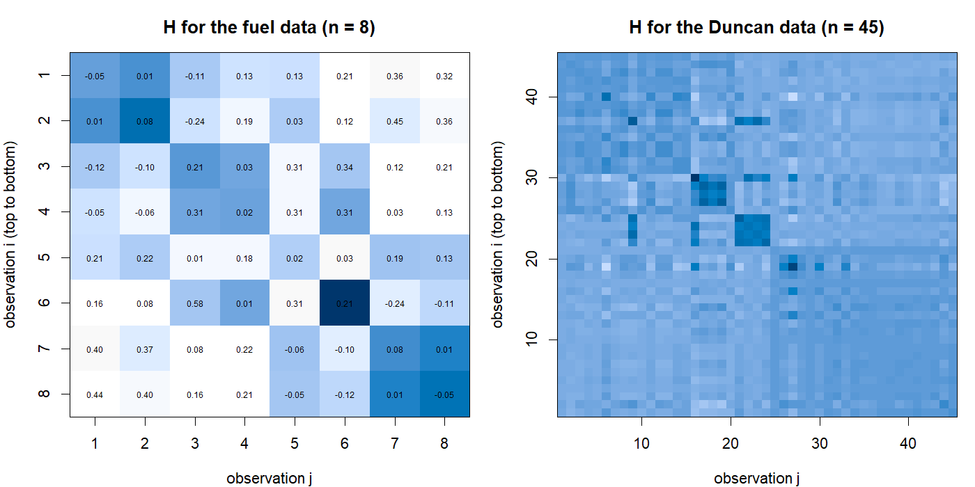
Hat matrix heatmap — 图：帽子矩阵热图 —— 杠杆值 h_ii 与成对影响 h_ij 的可视化

纯基础 R 代码（不依赖任何包）The R code: no packages

The complete script is MTH303_Ch3_Hat_Matrix_No_Packages.R. The essential extracts follow; each is three or four lines because $\bm H$ does all the work.

## --- the design matrix, built by hand (no model.matrix) -------------------
X <- cbind("(Intercept)" = rep(1, n), Temp = Temp, Chill = Chill)
y <- matrix(Fuel, ncol = 1)

XtX    <- t(X) %*% X
XtXinv <- solve(XtX)                 # (X'X)^-1
beta   <- XtXinv %*% t(X) %*% y      # least squares estimate

## --- THE HAT MATRIX, ALL OF IT --------------------------------------------
H <- X %*% XtXinv %*% t(X)
print(round(H, 5))                   # all n x n entries
h <- diag(H)                         # leverage

## --- fitted values and residuals ------------------------------------------
yhat <- H %*% y
e    <- y - yhat                     # same as (diag(n) - H) %*% y

## --- leverage, row by row, straight from the definition -------------------
h_rowwise <- sapply(1:n, function(i)
  as.numeric(t(X[i, , drop = FALSE]) %*% XtXinv %*% X[i, , drop = FALSE]))

## --- residual covariance structure ----------------------------------------
ImH <- diag(n) - H                   # Var(e) = sigma^2 (I - H)
var_e_factor <- diag(ImH)            # the 1 - h_ii

## --- MSE, standard errors, t tests, confidence intervals ------------------
k    <- ncol(X)
MSE  <- as.numeric(t(e) %*% e) / (n - k)
Vb   <- MSE * XtXinv                 # estimated Var(beta.hat)
se   <- sqrt(diag(Vb))
tv   <- as.numeric(beta) / se
tc   <- qt(0.975, n - k)
CI   <- cbind(as.numeric(beta) - tc * se, as.numeric(beta) + tc * se)

## --- standardised residual -------------------------------------------------
rstd <- as.numeric(e) / (sqrt(MSE) * sqrt(1 - h))

## --- studentised residual: BY REFITTING n times (no formula, no packages) --
rstu_refit <- sapply(1:n, function(i) {
  Xi <- X[-i, , drop = FALSE]; yi <- matrix(y[-i, ], ncol = 1)
  bi <- solve(t(Xi) %*% Xi) %*% t(Xi) %*% yi       # refit without obs i
  ei <- yi - Xi %*% bi
  s_i <- sqrt(as.numeric(t(ei) %*% ei) / (n - k - 1))
  e[i] / (s_i * sqrt(1 - h[i]))
})

## --- ... and the closed-form delete-one version ----------------------------
s_i   <- sqrt((as.numeric(t(e) %*% e) - as.numeric(e)^2 / (1 - h)) / (n - k - 1))
rstu  <- as.numeric(e) / (s_i * sqrt(1 - h))

## --- Cook's distance: definition (refit) and closed form -------------------
D_def <- sapply(1:n, function(i) {
  Xi <- X[-i, , drop = FALSE]; yi <- matrix(y[-i, ], ncol = 1)
  bi <- solve(t(Xi) %*% Xi) %*% t(Xi) %*% yi
  sum((yhat - X %*% bi)^2) / (k * MSE)
})
D <- (as.numeric(e)^2 / (k * MSE)) * h / (1 - h)^2

## --- delete-one change in the coefficients ---------------------------------
dbeta <- sapply(1:n, function(i)
  (XtXinv %*% matrix(X[i, ], ncol = 1) * as.numeric(e[i])) / (1 - h[i]))

## --- ANOVA, global F, partial F, prediction -------------------------------
ybar  <- mean(y)
TSS   <- as.numeric(t(y - ybar) %*% (y - ybar))
RegSS <- as.numeric(t(yhat - ybar) %*% (yhat - ybar))
RSS   <- as.numeric(t(e) %*% e)
Fstat <- (RegSS / (k - 1)) / (RSS / (n - k))

x0 <- matrix(c(1, 30, 10), ncol = 1)
se_mean <- sqrt(MSE * as.numeric(t(x0) %*% XtXinv %*% x0))
se_pred <- sqrt(MSE * (1 + as.numeric(t(x0) %*% XtXinv %*% x0)))

## --- heat map, base graphics ----------------------------------------------
pal <- hcl.colors(64, "Blues 3", rev = TRUE)     # dark = large
image(1:n, 1:n, t(H[n:1, ]), col = pal, zlim = c(0, max(abs(H))))

注记

Remark 52 (What is deliberately not used). Nothing in the list above calls hatvalues, rstandard, rstudent, cooks.distance, influence, vcov, confint, predict, anova or summary. Those appear only in the “CHECK against lm()” blocks, where they serve as an independent audit of the hand-built quantities. If you are teaching, keep that order: build first, check second.

所用公式清单Checklist of the formulas used

Quantity	Formula
Hat matrix	$\bm H=\bm X(\bm X^{\top}\bm X)^{-1}\bm X^{\top}$
Fitted values	$\hat{\bm y}=\bm H\bm y$
Residuals	$\bm e=(\bm I_n-\bm H)\bm y$
Leverage	$h_{ii}=[\bm H]_{ii}=\bm x_i^{\top}(\bm X^{\top}\bm X)^{-1}\bm x_i =\sum_jh_{ij}^{2}$
Leverage bounds	$0\le h_{ii}\le1$ , $\sum_ih_{ii}=k$ , $\bar h=k/n$
Residual covariance	$\operatorname{Var}(\bm e)=\sigma^{2}(\bm I_n-\bm H)$ , so $\operatorname{Var}(e_i)=\sigma^{2}(1-h_{ii})$
Coefficient covariance	$\operatorname{Var}(\hat{\bm\beta})=\sigma^{2}(\bm X^{\top}\bm X)^{-1}$ , estimated by $s^{2}(\bm X^{\top}\bm X)^{-1}$
Standard error	$\widehat{\mathrm{se}}(\hat\beta_j)=\sqrt{\mathrm{MSE}\,[(\bm X^{\top}\bm X)^{-1}]_{jj}}$
Standardised residual	$r_i=e_i/\bigl(s\sqrt{1-h_{ii}}\bigr)$
Studentised residual	$r_i^{*}=e_i/\bigl(s_{(i)}\sqrt{1-h_{ii}}\bigr)$ , $s_{(i)}^{2}=\dfrac{\mathrm{RSS}-e_i^{2}/(1-h_{ii})}{n-k-1}$
Delete-one fitted values	$\hat{\bm y}_{(i)}=\hat{\bm y}-\bm h_ie_i/(1-h_{ii})$
Delete-one coefficients	$\hat{\bm\beta}_{(i)}=\hat{\bm\beta}-(\bm X^{\top}\bm X)^{-1}\bm x_ie_i/(1-h_{ii})$
Cook’s distance	$D_i=\dfrac{e_i^{2}}{k\,s^{2}}\cdot\dfrac{h_{ii}}{(1-h_{ii})^{2}}$ , cut-off $4/(n-k)$
Sums of squares	$\mathrm{RSS}=\bm y^{\top}(\bm I_n-\bm H)\bm y$ , $\mathrm{Reg\,SS}=\bm y^{\top}\bigl(\bm H-\frac1n\bm 1\bm 1^{\top}\bigr)\bm y$
Total pull	$\sum_{ij}h_{ij}^{2}=\operatorname{tr}(\bm H)=k$

Files

File	Contents
`MTH303_Ch3_Hat_Matrix_` `No_Packages.R`	The script: 14 parts, every diagnostic rebuilt from $\bm H$
`MTH303_Ch3_Hat_Matrix_` `Output.txt`	Its complete output ( $551$ lines, $57$ successful checks)
`hat_matrix_heatmap.png`	The two heat maps, produced by the script
`MTH303_Ch3_Hat_Matrix_` `Handout.pdf`	This document
`MTH303_Ch3_MLR_Teaching_` `Notes.pdf`	The Chapter 3 notes this supplements

This bilingual teaching page was assembled by DeepSeek 4.1 Flash from the course LaTeX sources; the technical derivations are reproduced verbatim. 中文导读层由 DeepSeek 4.1 Flash 撰写，技术推导部分保留原始英文内容。

符号与模型Notation and the model

标量形式的模型The model in scalar form

矩阵形式的模型The model in matrix form

最小二乘估计Least squares estimation

最小二乘准则与正规方程The least squares criterion and the normal equations

拟合值、残差与帽子矩阵Fitted values, residuals and the hat matrix

估计量的均值与协方差Mean and covariance of the least squares estimator

ANOVA 表的完整推导The ANOVA table: derivations

第 1 步：ANOVA 恒等式Step 1: the ANOVA identity T S S = R e g S S + R S S

第 2 步：MSE 是 σ² 的无偏估计Step 2: M S E is an unbiased estimator of σ 2

第 3 步：RSS 与 RegSS 的分布及其独立性Step 3: distribution of R S S and R e g S S , and their independence

第 4 步：整体 F 检验Step 4: the global F -test

决定系数 R²The coefficient of determination

单个系数的推断与部分 F 检验Inference on a single coefficient, and the partial F -test

单个斜率的 t 检验与置信区间The t-test and confidence interval for one slope

一般线性（部分）F 检验The general linear (partial) F -test

回归诊断：杠杆、残差与影响Diagnostics: leverage, residuals and influence

杠杆值Leverage

残差方差与标准化残差Residual variance and standardised residuals

影响分析与 Cook 距离Influence and Cook’s distance

共线性与方差膨胀因子Collinearity and the variance inflation factor

手工计算的完整例题（燃料数据）Worked example computed by hand

数据The data

原始求和量The raw sums (everything else is built from these)

第 1 步：X'X 与 X'yStep 1: 𝑿 ⊤ 𝑿 and 𝑿 ⊤ 𝒚

第 2 步：X'X 的逆Step 2: the inverse of 𝑿 ⊤ 𝑿

The determinant.

The remaining cofactors and the inverse.

第 3 步：最小二乘估计Step 3: the least squares estimate

An exact cross-check worth doing once.

A second route, worth showing students.

第 4 步：拟合值、残差与正交性检验Step 4: fitted values, residuals and the orthogonality checks

第 5 步：三个平方和Step 5: the three sums of squares

第 6 步：ANOVA 表与整体 F 检验Step 6: the ANOVA table and the global F -test

第 7 步：标准误、t 检验与置信区间Step 7: standard errors, t -tests and confidence intervals

第 8 步：部分 F 检验与 t²=FStep 8: the partial F -test, and t 2 = F

第 9 步：本组数据的残差诊断Step 9: residual diagnostics for this data set

Worked detail for observation 4

第 10 步：新观测的预测Step 10: prediction for a new observation

去掉截距后有哪些变化What changes without an intercept

同一例题的 R 验证（逐项对照）The same example in R: side-by-side verification

模型与 ANOVA 表The model and the ANOVA table

手算与 R 的对照表The hand-versus-R comparison table

R 帮你算好的那些量The pieces R computes for you

教学安排与配套 R 脚本Teaching plan and the R script

Suggested 100-minute sequence

Common student errors to anticipate

The companion R script

Exercises

Matrix-calculus and trace facts used

Notation summary

References

补充讲义：帽子矩阵全解COMPANION_PART

帽子矩阵是什么、为什么叫“帽子矩阵”What 𝑯 is, and why it is called the hat matrix

燃料例题的完整 HThe complete 𝑯 for the fuel example

The matrix 𝑯\bm H — all 64 entries

The complement 𝑰n−𝑯\bm I_n-\bm H

H 的性质Properties of 𝑯

Numerical verification, from the script

杠杆值：从定义出发Leverage, from the definition

The fuel example

残差协方差矩阵 σ²(I−H)The residual covariance matrix σ 2 ( 𝑰 n − 𝑯 )

由 (X'X)⁻¹ 出发的标准误与推断Standard errors and inference, from ( 𝑿 ⊤ 𝑿 ) − 1

标准化残差与学生化残差Standardised and studentised residuals

The delete-one update formulas

The fuel example: closed form against actual refitting

Cook 距离Cook’s distance

The fuel example

完整影响分析表The full influence table

其余量都来自同一组矩阵Everything else, from the same matrices

更大规模的例子：Duncan 声望数据A larger case: Duncan prestige data, n = 45 , k = 5

帽子矩阵是什么、为什么叫“帽子矩阵”What the off-diagonal entries say

纯基础 R 代码（不依赖任何包）The R code: no packages

所用公式清单Checklist of the formulas used

Files

The matrix $\bm H$ — all 64 entries

The complement $\bm I_n-\bm H$